Wine Quality Prediction - Machine Learning

Here we will predict the quality of wine on the basis of given features. We use the wine quality dataset available on Internet for free. This dataset has the fundamental features which are responsible for affecting the quality of the wine. By the use of several Machine learning models, we will predict the quality of the wine.

Importing libraries and Dataset:

• Pandas is a useful library in data handling.
• Numpy library used for working with arrays.
• Seaborn/Matplotlib are used for data visualisation purpose.
• Sklearn - This module contains multiple libraries having pre-implemented functions to perform tasks from data preprocessing to model development and evaluation.
• XGBoost - This contains the eXtreme Gradient Boosting machine learning algorithm which is one of the algorithms which helps us to achieve high accuracy on predictions.

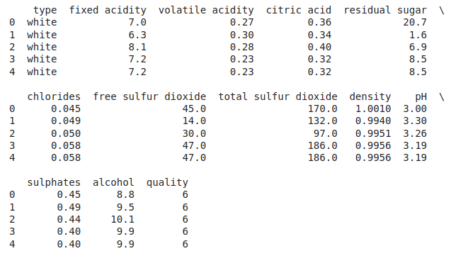
Now let's look at the first five rows of the dataset.

Output:

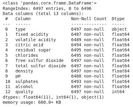
Let's explore the type of data present in each of the columns present in the dataset.

Output:

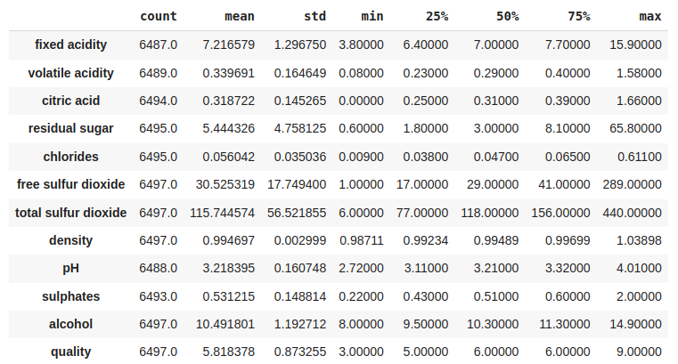
Now we'll explore the descriptive statistical measures of the dataset.

Output:

Exploratory Data Analysis

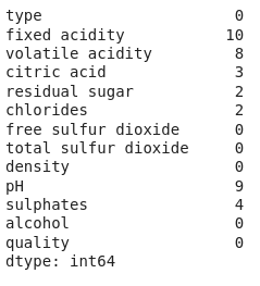
EDA is an approach to analysing the data using visual techniques. It is used to discover trends, and patterns, or to check assumptions with the help of statistical summaries and graphical representations.  Now let's check the number of null values in the dataset columns wise.

Output:

Let's impute the missing values by means as the data present in the different columns are continuous values.

Output:

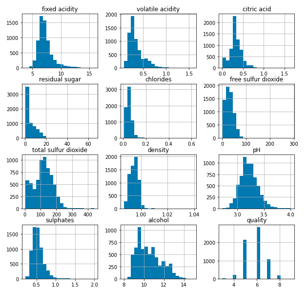
0

Let's draw the histogram to visualise the distribution of the data with continuous values in the columns of the dataset.

Output:

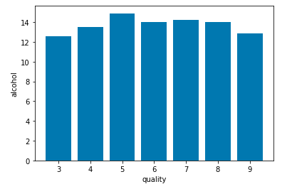
Now let's draw the count plot to visualise the number data for each quality of wine.

Output:

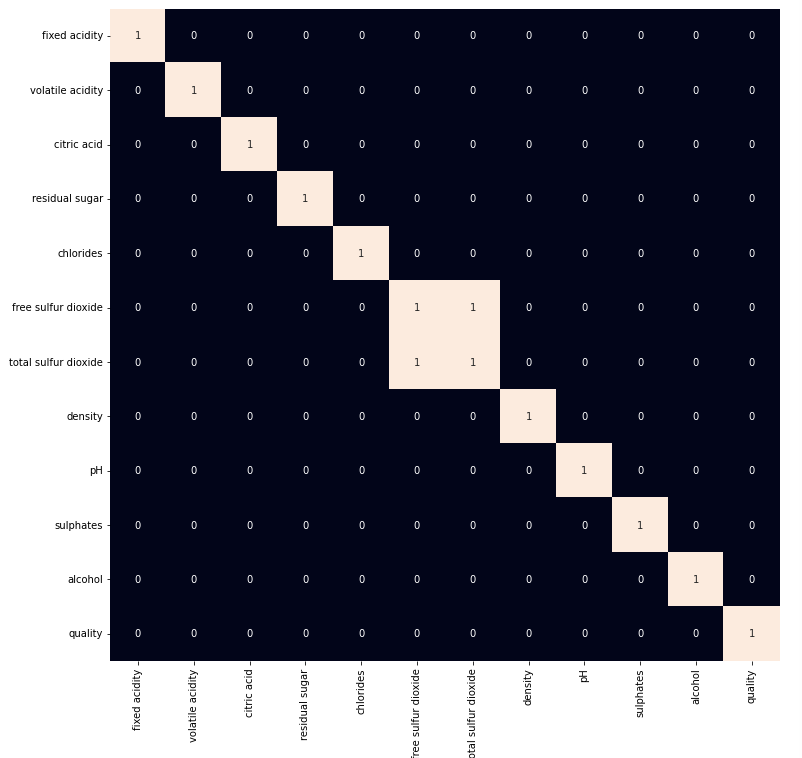
There are times the data provided to us contains redundant features they do not help with increasing the model's performance that is why we remove them before using them to train our model.

Output:

From the above heat map we can conclude that the 'total sulphur dioxide' and 'free sulphur dioxide' are highly correlated features so, we will remove them.

Model Development

Let's prepare our data for training and splitting it into training and validation data so, that we can select which model's performance is best as per the use case. We will train some of the state of the art machine learning classification models and then select best out of them using validation data.

We have a column with object data type as well let's replace it with the 0 and 1 as there are only two categories.

After segregating features and the target variable from the dataset we will split it into 80:20 ratio for model selection.

Output:

((5197, 10), (1300, 10))

Normalising the data before training help us to achieve stable and fast training of the model.

As the data has been prepared completely let's train some state of the art machine learning model on it.

Output:

LogisticRegression() : 
Training Accuracy : 0.6975101024661644
Validation Accuracy : 0.6855058693719925

XGBClassifier() : 
Training Accuracy : 0.9762240429934201
Validation Accuracy : 0.8045662590288206

SVC() : 
Training Accuracy : 0.7203202525576721
Validation Accuracy : 0.7073819229472522

Model Evaluation

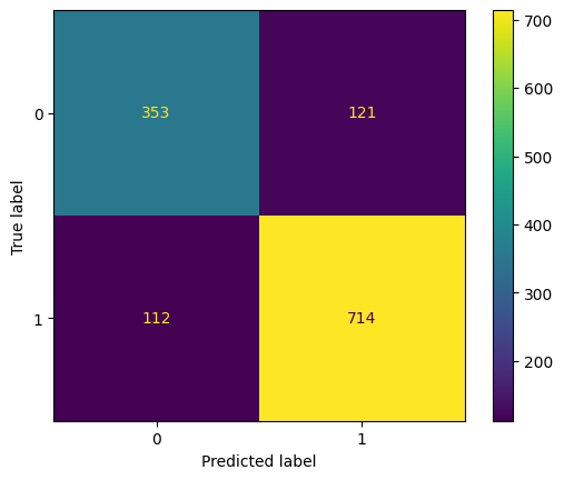
From the above accuracies we can say that Logistic Regression and SVC() classifier performing better on the validation data with less difference between the validation and training data. Let's plot the confusion matrix as well for the validation data using the Logistic Regression model.

Output:

Let's also print the classification report for the best performing model.

Output:

 precision recall f1-score support

 0 0.76 0.74 0.75 474
 1 0.86 0.86 0.86 826

 accuracy 0.82 1300
 macro avg 0.81 0.80 0.81 1300
weighted avg 0.82 0.82 0.82 1300

Get the Complete Notebook

Notebook: click here.

Dataset : click here.