Advanced OpenCV and NumPy Operations: Cropping, Copying, And Pasting

This article was published as a part of the Data Science Blogathon

Introduction

Computer Vision is a real-world application of Machine Learning, that provides computers with the ability to see and identify physical 3D objects in real-time. Computer Vision plays an extremely important role when a robot is required to be autonomous in its navigation and mobility. Computer Vision allows us to indulge in high-level computation and processing tasks.

If you have not read through my previous articles on Computer Vision and OpenCV and would like to do so, please navigate to the following hyperlinks:

• : An Introduction to Computer Vision With OpenCV
• : Performing Computer Vision Task With OpenCV And Python
• : Some Advanced OpenCV Operations For Your Computer vision Project
• : Some Advanced OpenCV Functions For Your Computer Vision Project Continued
• : Beginner’s Guide to Python OpenCV Operation: Rotation

This article will aim to introduce us to more features pertaining to the OpenCV package in Python Programming Language. To facilitate this particular learning process, we will attempt to perform our OpenCV Operations on an image that may be downloaded from this link. Alternatively, you may save the image found below.

Source: The Humble I.

Getting Started

At this point in our OpenCV learning experience, we should by now, be familiar with the first and foremost task to perform- That is, the task of loading the image into our system memory-
and to do so, we are required to import the necessary packages into our system
memory. The importation and loading code is as follows:

# import the required packages
import cv2
import os
import numpy as np

# load the image into system memory
image = cv2.imread('C:/Users/Shivek/Pictures/Nature.jpg', flags=cv2.IMREAD_COLOR)
cv2.imshow('Analytics Vidhya Computer Vision- Nature', image)
cv2.waitKey()
cv2.destroyAllWindows()

The main points to note in the above code blocks are as follows:

• We imported the necessary python packages into our system memory.
• We made use of the imread() method to facilitate the process of loading data (the image) from the Hard Disk Drive into our system RAM.
• We load the image in default/standard format, i.e., color format.

Output to the above code blocks will be seen as follows:

The image looks good! However, on the vast plain, we can see, there
exists only one tree. Let us fix this using OpenCV and NumPy techniques.

Cropping An Image

The technique of cropping involves making physical adjustments to an image using digital means. Cropping is useful in times of isolating the required portion of an image from the rest, or for bringing the attention of the viewer to a particular area of the image.

As we already know, OpenCV represents an image as a NumPy array comprising integers that represent the pixels and intensity- hence, by indexing and slicing portions of the NumPy array, we are essentially isolating specific pixels thereby isolating specific portions of the image itself, thus allowing us to effectively crop the image.

Since cropping an image requires indexing and slicing, it is important that we know the shape of our matrix, i.e., NumPy array. This is because we will use the index values to perform this task.

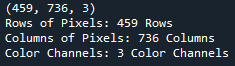
print(image.shape)
print("Rows of Pixels: %d Rows"%(image.shape[0]))
print("Columns of Pixels: %d Columns"%(image.shape[1]))
print("Color Channels: %d Color Channels"%(image.shape[2]))

Output to the above lines of code will show as follows:

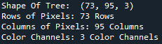
From the above image, one is able to see that our image has the
following properties:

• 459 Rows of Pixels.
• 736 Columns of Pixels.
• 3 Color Channels- By Default BGR is used, not RGB. You will find that the Red and Blue color channels have been swapped.

As we have seen previously, our downloaded image shows a geographical plain, which has a single tree. The image looks good, but we will attempt to populate the plain with a few more trees.

Add more trees to the plain.

It is good to keep in mind that we are working with arrays- although it is an image- it is in the form of an array. With an array, we are able to , and . Essentially, what we aim to do is , and thereafter .

To explain the above methodology, allow me to provide you with a small-scale example.

Example of our objective

Here is a small example to explain the process that we will be performing, to you.

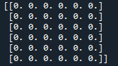
We will import NumPy, and create an array of zeros with dimensions 6 rows and 6 columns representing the original image. We will print the array of zeros to the console.

import numpy as np
numpy_zeros = np.zeros(shape=(6, 6))
print(numpy_zeros)

Our NumPy array of zeros is as below:

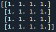
Next, we will create an array of ones with dimensions 4 row and 4 columns representing the tree. We will print the array of ones to the console.

numpy_ones = np.ones(shape=(4, 4))
print(numpy_ones)

The output will be seen as follows:

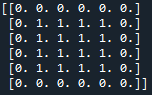
Now, we will . We will select the portion of values using slicing techniques. It is good to know that the size of the array you are imputing values into, must be the same size as the array with the values to be imputed.

numpy_zeros[1:5, 1:5] = numpy_ones
print(numpy_zeros)

Output to the above block of code will be seen as below:

And we have successfully manipulated our array. The process of cropping works in a similar way- I do hope that you have a better understanding of the process. Let’s scale it up!

Coming Back To OpenCV

So our objective is to find the pixel array that makes up the tree, isolate this pixel array, and make portions of the original array be equal to the tree pixel array. It sounds difficult, but it is not and is very interesting.

We begin by finding the matrix that comprises the tree as below:

tree = image[320:393, 570:665]
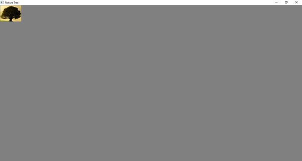
cv2.imshow('Nature Tree', tree)
cv2.waitKey()
cv2.destroyAllWindows()

Let us display the output of the above pixels to the screen- Output will be seen as follows:

• The image is as it should be.
• The gray-colored area is visible because the image is small.
• There is no title bar visible due to the size of the image.
• If you would like to see the image in a full window, you may maximize the window and upon which doing, you will be presented with the below output:

Let us view the shape of the pixel array:

print('Shape Of Tree: ', tree.shape)
print("Rows of Pixels: %d Rows"%(tree.shape[0]))
print("Columns of Pixels: %d Columns"%(tree.shape[1]))
print("Color Channels: %d Color Channels"%(tree.shape[2]))

The output to the above code block will be seen as follows:

Now that we have the pixel array of the tree, as well as the size of the array, we can set array portions in the original image to be equal to the tree
pixel array- Remember that both pixel arrays need to be the same size.

image[333:406, 0:95] = tree
image[333:406, 95:190] = tree[:, ::-1, :]
image[323:396, 190:285] = tree[:, ::-1, :]
image[323:396, 285:380] = tree[:, :, :]
image[312:385, 380:475] = tree[:, ::-1, :]
image[315:388, 475:570] = tree

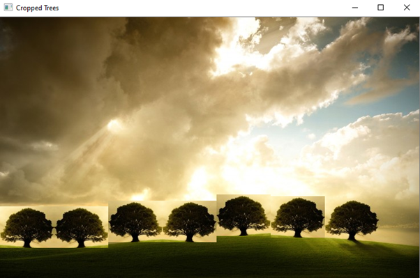
Now let us display the original image to the screen. We expect to find more trees in our image:

cv2.imshow('Cropped Trees', image)
 cv2.waitKey()
 cv2.destroyAllWindows()

Output to the above code block will show as follows:

And thus, we have successfully cropped the tree from our image and added more trees to the original image, using a method of Copying And Pasting.

This concludes my article on I do hope that you found this article enlightening and interesting and have new takeaways of the OpenCV package in Python.

Please feel free to connect with me on LinkedIn. If you would like to see all articles that I have composed for Analytics Vidhya, please navigate to my Analytics Vidhya Profile.

Thank you for your time.

I would like to thank the reader for taking the
time to read my article up to this point, as from my view, it is one of the most detailed and
time-consuming articles that I have written. I hope you have learned a new
concept about OpenCV Operations- .

Login to continue reading and enjoy expert-curated content.

Free Courses