Convolutional Neural Networks (CNNs) are deep learning models designed to analyze structured grid-like data such as images. They learn visual patterns directly from pixel values and identify features like edges, textures, shapes and objects. In R, CNN models can be built using libraries such as Keras and TensorFlow for tasks like image classification and object recognition.
CNNs learn visual features automatically from images, starting with simple patterns like edges and textures and gradually learning more complex shapes and objects in deeper layers.
Convolution operations capture spatial relationships between neighboring pixels, allowing the model to understand patterns and structures present in visual data.
By sharing weights and focusing on local regions of an image, CNNs reduce the number of parameters and can recognize the same feature even if it appears in different positions.
Key Components of Convolutional Neural Networks (CNN)
A Convolutional Neural Network (CNN) is composed of multiple layers, where each layer transforms the input data to extract increasingly complex features. These layers work together to learn patterns from images and perform tasks such as classification or object detection.
1. Input Layer
The input layer receives the raw image data and passes it to the network for further processing.
Accepts image data in the form of a 3D volume (width × height × depth).
Stores pixel intensity values of the image.
Preserves the spatial structure of the image for feature extraction in later layers.
Example: For an RGB image of size 32 × 32, the input volume becomes 32 × 32 × 3, where 3 represents the color channels (Red, Green, Blue).
2. Convolutional Layer
The convolutional layer extracts important visual patterns from the input using learnable filters.
Applies small filters that slide across the input image.
Performs element-wise multiplication between filter values and image patches.
Generates feature maps that capture patterns such as edges, textures and shapes.
Example: If 12 filters are applied to a 32 × 32 × 3 image, the output feature map volume may become 32 × 32 × 12.
3. Activation Layer
The activation layer introduces non-linearity into the network, allowing it to learn complex patterns.
Connects every neuron from the previous layer to neurons in the current layer.
Performs high-level reasoning using learned features.
Often used near the end of the CNN architecture.
Example: The 3072-length vector from the flattening layer is connected to neurons that compute classification scores.
7. Dropout Layer
The dropout layer is used as a regularization technique to reduce overfitting during training.
Randomly disables a fraction of neurons during each training iteration.
Forces the network to learn more robust and generalized features.
Improves the model’s ability to perform well on unseen data.
Example: A dropout rate of 0.5 randomly deactivates 50% of neurons during training to prevent the model from relying too heavily on specific neurons.
8. Output Layer
The output layer produces the final prediction of the CNN model.
Converts the network output into probability values.
Uses activation functions depending on the task.
Provides the final classification or prediction result.
Example: For a 10-class classification problem, the Softmax function outputs 10 probability values, each representing the likelihood of a class.
How CNN Works
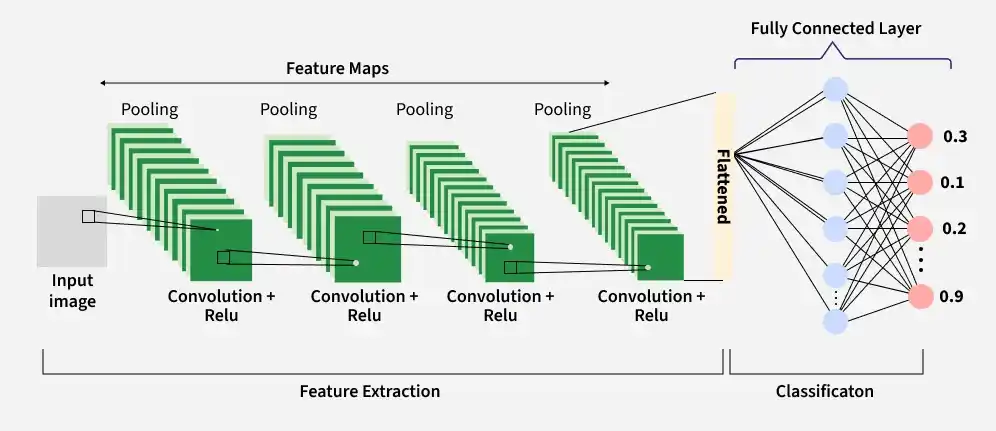
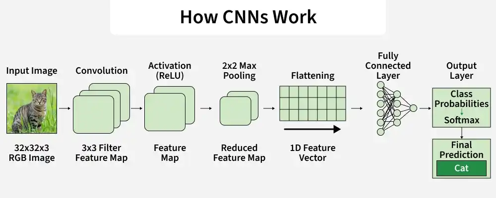
A Convolutional Neural Network processes an image through multiple layers to gradually extract features and make a final prediction. The process begins with the raw image as input and passes through convolution, activation, pooling and fully connected layers before producing the final output.
Step 1: The CNN receives the raw image as input in the form of a three-dimensional matrix representing width, height and color channels (RGB). This structure stores pixel intensity values while preserving the spatial arrangement of the image for feature learning.
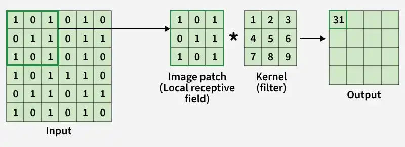
Step2: The convolution layer extracts important features from the input image using filters (kernels).
A small matrix called a filter or kernel slides over the image.
At each position, the filter performs element-wise multiplication with the corresponding image patch.
The multiplied values are summed together to produce a single value in the output.
Step 3: The convolution operation applies filters that move across the image using a defined stride to detect patterns. The output produced is called a feature map and multiple filters are used to capture different features such as edges, textures and shapes.
Step4: After convolution, an activation function is applied to introduce non-linearity, allowing the model to learn complex patterns from the feature maps. The most commonly used activation function in CNNs is ReLU (Rectified Linear Unit).
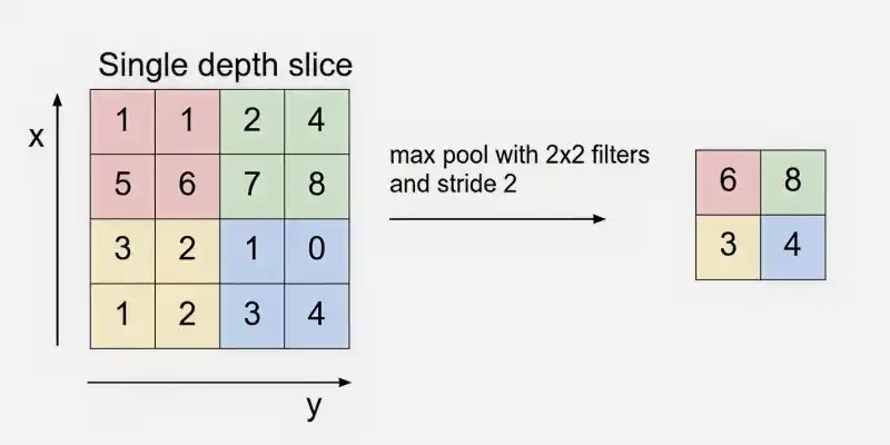
Step 5: Next, a pooling operation is applied the spatial dimensions of the feature maps while retaining important information.
Step 6: In CNNs, convolution and pooling layers are repeated multiple times to learn deeper and more complex features. Early layers detect simple patterns like edges, while deeper layers capture textures, shapes and complex objects.
Step 7: Next, flattening converts the multi-dimensional feature maps produced by convolution and pooling layers into a one-dimensional vector.
Step 8: After flattening, the extracted features are passed to the fully connected layer, which performs high-level reasoning and produces the final prediction through the output layer.
The fully connected layer connects neurons from the previous layer and combines learned features for classification.
The output layer converts the final scores into probabilities using Sigmoid for binary classification or Softmax for multi-class classification.
Step By Step Implementation
Here we implement Convolutional Neural Network (CNN) in R using Keras and TensorFlow.
Step 1: Installing the required packages
Install and load the Keras library in R, which provides an interface for building deep learning models. The install_keras() function automatically installs the required TensorFlow backend and configures the Python environment needed to run neural networks.
Define the CNN architecture by stacking convolutional, pooling, flattening and fully connected layers to extract features and perform classification.
layer_conv_2d(): Adds convolutional layers to detect features such as edges, textures and shapes.
layer_max_pooling_2d(): Reduces spatial dimensions and controls overfitting by keeping important features.
layer_flatten(): Converts multi-dimensional feature maps into a 1D vector for fully connected layers.
layer_dense() and layer_dropout(): Fully connected layers perform classification, with dropout used to prevent overfitting.
Output layer (softmax): Produces probabilities for each of the 10 digit classes.
Step 7: Compiling and Training the CNN
Here we compile the CNN with an optimizer, loss function and metrics, then train it on the dataset while monitoring validation performance.
optimizer_adam(): Uses the Adam optimizer, which adapts the learning rate for faster and efficient training.
categorical_crossentropy: Loss function for multi-class classification with one-hot encoded labels.
c('accuracy'): Metric used to evaluate model performance during training.
epochs: Number of times the entire dataset is passed through the model.
batch_size: Number of samples processed before updating the model weights.
validation_split: Training data reserved for validation to monitor performance on unseen data.
Step 8: Evaluating the CNN Model
Trained CNN is evaluated on the test dataset to measure its final performance in terms of loss and accuracy on unseen data.
Output:
loss accuracy
0.05012181 0.98710001
Test loss: 0.05012181
Test accuracy: 0.9871
Step 9: Visualizing Training History
Here we plot the training and validation accuracy and loss over epochs to monitor the model’s learning progress and detect overfitting or underfitting.
