Dog Breed Classification using Transfer Learning

In this tutorial, we will demonstrate how to build a dog breed classifier using transfer learning. This method allows us to use a pre-trained deep learning model and fine-tune it to classify images of different dog breeds.

Why to use Transfer Learning for Dog Breed Classification

Transfer learning is a machine learning technique where a pre-trained model, which has been trained on a large dataset, is adapted to a new task.

For example, models trained on ImageNet can be reused for other tasks like dog breed classification. The key advantage of transfer learning is that it allows us to utilize the feature-extraction capabilities of a model that has already learned useful representations from millions of images. By reusing the convolutional layers of these models, we can achieve high accuracy with less training data and reduced computational effort.

Benefits of Transfer Learning in Dog Breed Classification

• Faster Training: Pre-trained models have already learned to identify key image features, saving time on training.
• Improved Accuracy: Using a pre-trained model on a similar task helps in achieving better performance than training from scratch.
• Less Data Requirement: Transfer learning requires fewer data for fine-tuning, making it ideal for tasks like dog breed classification where labeled data might be limited.

Implementing Dog Breed Classification using Transfer Learning

Step 1: Import Necessary Libraries

To implement this project, we will use the following Python libraries, each suited for specific tasks such as data handling, model development, and image processing:

• Pandas: For data manipulation and preprocessing.
• Numpy: For numerical computations and array manipulations.
• Matplotlib and Seaborn: For visualizing the dataset and model performance.
• Scikit-learn (Sklearn): For data preprocessing, splitting datasets, and model evaluation.
• OpenCV: For image processing tasks such as resizing, cropping, and converting images.
• TensorFlow and Keras: For building and training the deep learning model using transfer learning.

Step 2: Loading Dataset for Dog Breed Classification

The dataset contains 10,000 images of 120 different dog breeds. The dataset includes:

• Training images: Contains labeled images of dog breeds.
• Test images: Unlabeled images used for testing the model.
• CSV file: Contains metadata about the images and their corresponding dog breed labels.

You can access the dataset here: Dog Breed Identification Dataset

To start using the dataset, we will unzip the file to extract the contents.

Output:

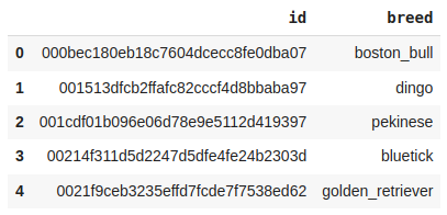
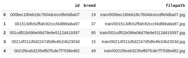
The data set has been extracted.

Step 3: Exploratory Data Analysis

Now that we have the dataset, let's perform some basic Exploratory Data Analysis (EDA).

Output:

Output:

(10222, 2)

Let's check the number of unique breeds of dog images we have in the training data.

Output:

120

So, here we can see that there are 120 unique breed data which has been provided to us.

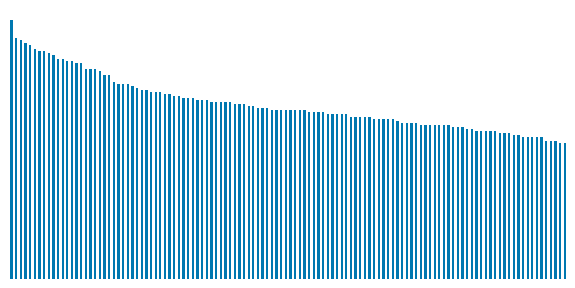
Output:

Here we can observe that there is a data imbalance between the classes of different breeds of dogs.

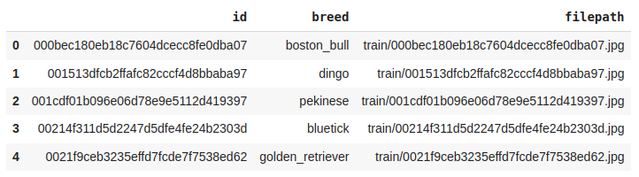
Output:

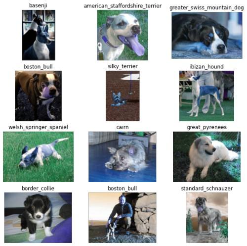
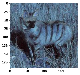
Although visualizing one image from each class is not feasible but let's view some of them.

Output:

The images are not of the same size which is natural as real-world images tend to be of different sizes and shapes. We will take care of this while loading and processing the images.

Output:

Step 4: Data Preparation

When working with large datasets in deep learning, memory limitations often prevent loading the entire dataset at once. To efficiently handle data loading and augmentation, tools like TensorFlow’s tf.data.Dataset and Albumentations are used to create optimized input pipelines and apply real-time image augmentations.

First, the dataset is split into training and validation sets, enabling model training on one subset and evaluation on another.

Output:

((8688,), (1534,))

Step 5: Applying Image Augmentation

Below are some of the augmentations which we would like to have in our training data.

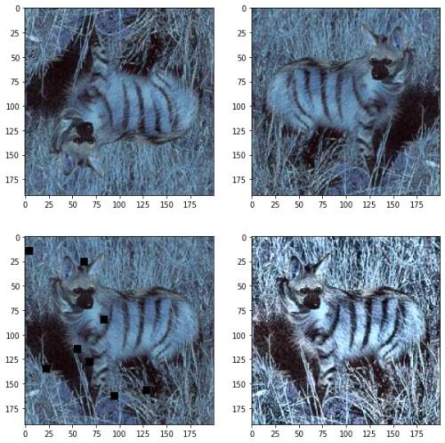
Let's view an example of albumentation by applying it to some sample images.

Output:

Next, we apply several augmentations, such as VerticalFlip, HorizontalFlip, CoarseDropout, and CLAHE, and visualize the results:

Output:

Different augmentations applied to the sample image, showing how the data transformation looks visually.

Step 6: Building the Input Pipeline

Now, let's define utility functions to handle image loading, augmentation, and normalization. We will create functions to read images from disk, resize them, normalize the pixel values, and apply augmentations.

Below we have implemented some utility functions which will be used while building the input pipeline.

• decode_image: This function will read the image from the path and resize them to be of the same size along with it will normalize as well. Finally, we will convert the labels into one_hot vectors as well.
• process_data: This is the function that will be used to introduce image augmentation to the image.

Now by using the above function we will be implementing our training data input pipeline and the validation data pipeline.

We must observe here that we do not apply image data augmentation on validation or testing data.

Output:

(32, 128, 128, 3) (32, 120)

From here we can confirm that the images have been converted into (128, 128) shapes and batches of 64 images have been formed.

Step 7: Model Building Using Transfer Learning

1. Load Pre-trained InceptionV3 Model

We first load the InceptionV3 model from TensorFlow's Keras API with the weights pre-trained on ImageNet. The include_top=False argument excludes the fully connected layers at the top of the network, allowing us to customize the final layers for our task.

Output:

87916544/87910968 [==============================] - 1s 0us/step
87924736/87910968 [==============================] - 1s 0us/step

The model is successfully loaded with the weights from ImageNet, and we can now access the feature extraction layers.

2. Inspect the Model's Depth

InceptionV3 is a deep network with many layers, which makes it effective in learning complex features from images. Let's check the number of layers in this pre-trained model.

Output:

311

This deep architecture, consisting of 311 layers, makes it highly efficient at extracting detailed features from images.

3. Freeze Pre-Trained Layers

Since the convolutional layers of the InceptionV3 model have already been trained on millions of images, we freeze these layers so that their weights are not updated during our fine-tuning process.

Output:

last layer output shape: (None, 6, 6, 768)

This tells us that the last convolutional layer outputs a 6x6 grid of feature maps with 768 channels.

5. Define the Custom Model Architecture

Using the Keras Functional API, we can build a custom classification head on top of the pre-trained model. This includes flattening the output, adding fully connected layers, BatchNormalization for stable training, Dropout for regularization, and finally, an output layer with softmax activation for multi-class classification.

6. Implement Callbacks

Callbacks are used to monitor the model's performance during training. We use the following callbacks:

• EarlyStopping: Stops training if validation AUC doesn't improve for 3 consecutive epochs, preventing overfitting.
• ReduceLROnPlateau: Reduces the learning rate when the validation loss plateaus, helping the model converge better.
• Custom Callback: Stops training if the validation AUC exceeds 0.99.

Step 8: Train the Model

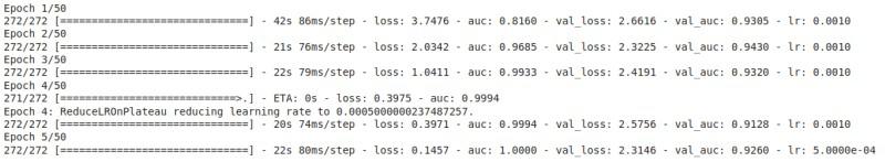
We train the model using the fit() method with training and validation datasets, a maximum of 50 epochs, and the callbacks defined above.

Output:

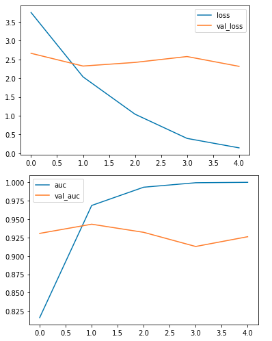
The output will display the training and validation loss, as well as the AUC score after each epoch. If the validation AUC exceeds 0.99, the training will stop early.

Step 9: Evaluate the Model

Once the model is trained, we evaluate its performance on the test dataset. We visualize the training history to observe the model's learning curve and make sure it has converged effectively.

Output:

The training and validation AUC curves are plotted, showing how the model's performance evolved over time. The test loss and test AUC are displayed, providing insight into how well the model generalizes to unseen data.

Source Code: Dog Breed Classification