Multiclass image classification using Transfer learning

Image classification is one of the supervised machine learning problems which aims to categorize the images of a dataset into their respective categories or labels. Classification of images of various dog breeds is a classic image classification problem. So, we have to classify more than one class that's why the name multi-class classification, and in this article, we will be doing the same by making use of a pre-trained model InceptionResNetV2, and customizing it.

Let's first discuss some of the terminologies.

Transfer learning: Transfer learning is a popular deep learning method that follows the approach of using the knowledge that was learned in some task and applying it to solve the problem of the related target task. So, instead of creating a neural network from scratch we "transfer" the learned features which are basically the "weights" of the network. To implement the concept of transfer learning, we make use of "pre-trained models".

Necessities for transfer learning: Low-level features from model A (task A) should be helpful for learning model B (task B).

Pre-trained model: Pre-trained models are the deep learning models which are trained on very large datasets, developed, and are made available by other developers who want to contribute to this machine learning community to solve similar types of problems. It contains the biases and weights of the neural network representing the features of the dataset it was trained on. The features learned are always transferrable. For example, a model trained on a large dataset of flower images will contain learned features such as corners, edges, shape, color, etc.

InceptionResNetV2: InceptionResNetV2 is a convolutional neural network that is 164 layers deep, trained on millions of images from the ImageNet database, and can classify images into more than 1000 categories such as flowers, animals, etc. The input size of the images is 299-by-299.

Dataset description:

• The dataset used comprises of 120 breeds of dogs in total.
• Each image has a file name which is its unique id.
• : contains 10,222 images which are to be used for training our model
• : contains 10,357 images which we have to classify into the respective categories or labels.
• : contains breed names corresponding to the image id.
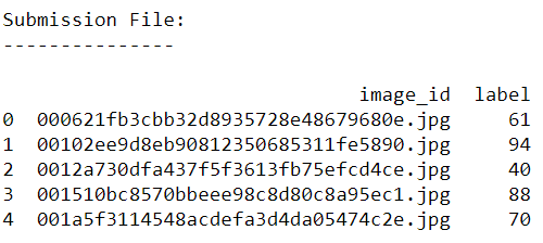
• : contains correct form of sample submission to be made

All the above mentioned files can be downloaded from .

: For better performance use GPU.

We first import all the necessary libraries.

Loading datasets and image folders

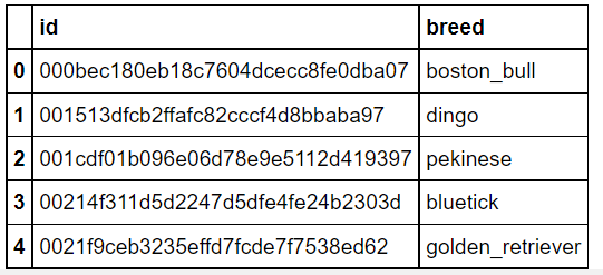
Displaying the first five records of labels dataset to see its attributes.

Output: 

👁 Image

Adding '.jpg' extension to each id 

This is done in order to fetch the images from the folder since the image name and id's are the same so adding .jpg extension will help us in retrieving images easily.

Augmenting data:

It's a pre-processing technique in which we augment the existing dataset with transformed versions of the existing images. We can perform scaling, rotations, increasing brightness, and other affine transformations. This is a useful technique as it helps the model to generalize the unseen data well.

ImageDataGenerator class is used for this purpose which provides a real-time augmentation of data.a 

Description of few of its parameters that are used below:

• rescale: rescales values by the given factor
• horizontal flip: randomly flip inputs horizontally.
• validation_split: this is the fraction of images reserved for validation (between 0 and 1).

Output:  

👁 Image

Let's see what a single batch of data looks like.

Output: 

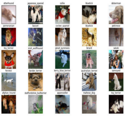
(32, 331, 331, 3)

Plotting images from the train dataset

Output:   

👁 Image

Building our Model

This is the main step where the neural convolution model is built.

BatchNormalization :

• It is a normalization technique which is done along mini-batches instead of the full data set.
• It is used to speed up training and use higher learning rates.
• It maintains the mean output close to 0 and the output standard deviation close to 1.

GlobalAveragePooling2D :

• It takes a tensor of size (input width) x (input height) x (input channels) and computes the average value of all values across the entire (input width) x (input height) matrix for each of the (input channels).
• The dimensionality of the images is reduced by reducing the number of pixels in the output from the previous neural network layer.
• By using this we get a 1-dimensional tensor of size (input channels) as our output.
• 2D Global average pooling operation. Here 'Depth' = 'Filters'

Dense Layers: These layers are regular fully connected neural network layers connected after the convolutional layers.

Drop out layer: is also used whose function is to randomly drop some neurons from the input unit so as to prevent overfitting. The value of 0.5 indicates that 0.5 fractions of neurons have to be dropped.

Compile the model:

Before training our model we first need to configure it and that is done by model.compile() which defines the loss function, optimizers, and metrics for prediction.

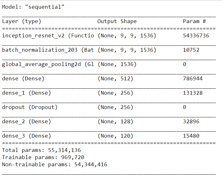
Displaying a summary report of the model

By displaying the summary we can check our model to confirm that everything is as expected.

Output:  

👁 Image

Defining callbacks to preserve the best results:

Callback: It is an object that can perform actions at various stages of training (for example, at the start or end of an epoch, before or after a single batch, etc).

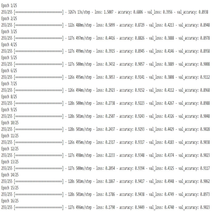
Training the model: It means that we are finding a set of values for weights and biases that have a low loss on average across all the records.

Output: 

👁 Image

Save the model

We can save the model for further use.

Visualizing the model's performance

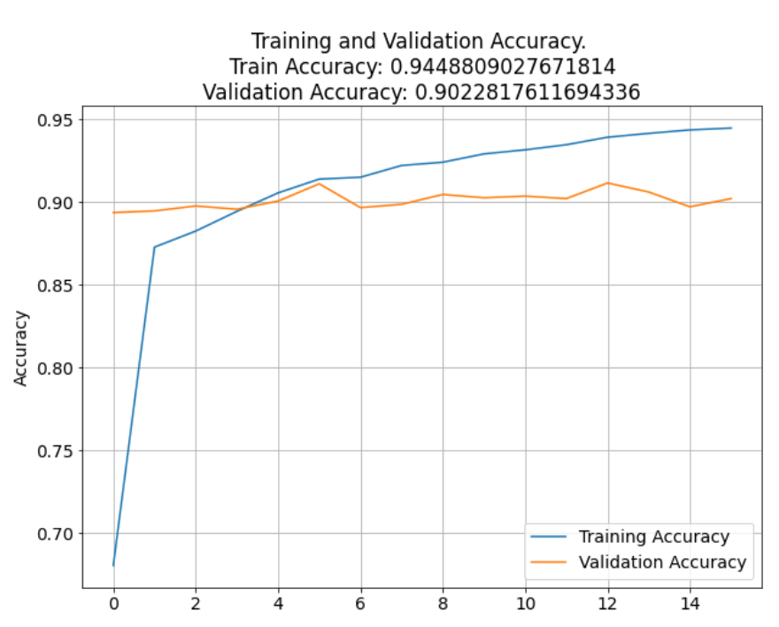
Output:  Text(0.5, 1.0, '\nTraining and Validation Accuracy. \nTrain Accuracy: 0.9448809027671814\nValidation Accuracy: 0.9022817611694336')

👁 Image

Output:   

👁 Image

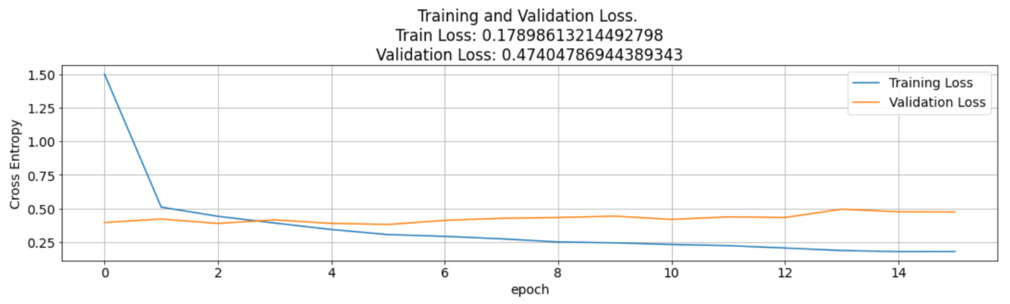
A line graph of training vs validation accuracy and loss was also plotted. The graph indicates that the accuracies of validation and training were almost consistent with each other and above 90%. The loss of the CNN model is a negative lagging graph which indicates that the model is behaving as expected with a reducing loss after each epoch.

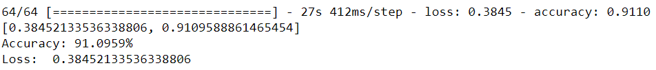
Evaluating the accuracy of the model

Output: 

👁 Image

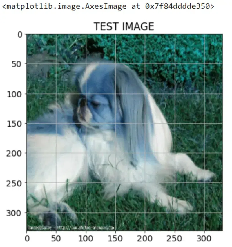
Viewing the Test Image

Output:

Making predictions on the test data

Output: 

👁 Image

Get the complete notebook link here

Colab Link : click here.

Dataset Link : click here.