To learn efficient data representations with minimal redundancy, Sparse Autoencoders play an important role in deep learning. They are a special type of autoencoder that introduces a sparsity constraint on the hidden layer, forcing only a few neurons to activate at a time.
Restricts hidden layer activation so the network focuses only on the most informative features.
Prevents the autoencoder from overfitting or copying inputs directly.
Helps extract meaningful structure from high-dimensional data.
The sparsity is typically controlled through regularization techniques like L1 penalty or KL divergence.
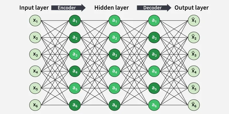
The diagram shows a sparse autoencoder with an encoder-decoder structure, where the hidden layer learns a compressed internal representation by keeping most hidden units inactive (sparse).
Importance of Sparse Autoencoders
Sparse autoencoders are useful for learning compact and meaningful representations of data without supervision.
Feature Learning: Extracts important features from unlabeled data for tasks like classification and clustering.
Dimensionality Reduction: Compresses high dimensional data while preserving essential information.
Anomaly Detection: Identifies unusual inputs that deviate from learned patterns.
Denoising: Reconstructs clean data from noisy inputs.
Pretraining Networks: Provides a strong weight initialization for deep networks.
Interpretable Representations: Sparse activations highlight the most informative features.
How it Works
Sparse autoencoders combine an encoder, decoder and sparsity constrained loss function to learn compact meaningful representations. The loss function used is:
where
: Input data
: Reconstructed output
: Regularization parameter
: A function penalizing deviations from sparsity
Working:
Encoder compresses the input into a low dimensional latent representation.
Decoder reconstructs the input from the encoded features.
Sparsity Constraint ensures only a small number of hidden neurons activate for each input.
Methods to Enforce Sparsity
Sparsity is enforced to ensure the autoencoder learns high level features by activating only a small subset of neurons
L1 Regularization: Applies a penalty proportional to the absolute activations or weights, encouraging the network to use fewer neurons.
KL Divergence: Measures how far the average activation deviates from the target sparsity level, ensuring that only a subset of neurons activates at a time.
Sparsity Proportion: Defines the desired activation frequency of hidden units across training samples.
How Sparse Autoencoders Are Trained
Training a sparse autoencoder follows the same workflow as a standard autoencoder but includes an additional step to enforce sparsity on the hidden layer:
1. Initialization: The network weights are initialized randomly or using pre-trained models to provide a stable starting point.
2. Forward Pass: Input data is passed through the encoder to obtain the latent (compressed) representation and then through the decoder to reconstruct the original input.
3. Loss Calculation: The total loss combines:
Reconstruction error: MSE between and
Sparsity penalty: Uses KL Divergence or L1 regularization to keep most hidden units inactive.
4. Backpropagation and Optimization: Gradients are computed from the combined loss and used to update the network weights, ensuring the model learns both accurate reconstruction and sparse feature representations.
Step-By-Step Implementation
Here builds a Sparse Autoencoder using TensorFlow and Keras to learn compressed, sparse feature representations. The network is designed to learn compressed and sparse feature representations of the input data, enabling efficient encoding while retaining important information.
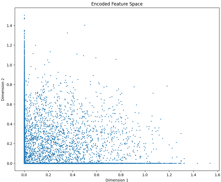
The scatter plot visualizes the 2-dimensional encoded feature space learned by the autoencoder. It shows how input samples cluster after compression, with many points near zero, indicating sparse activations typical of sparse autoencoders.
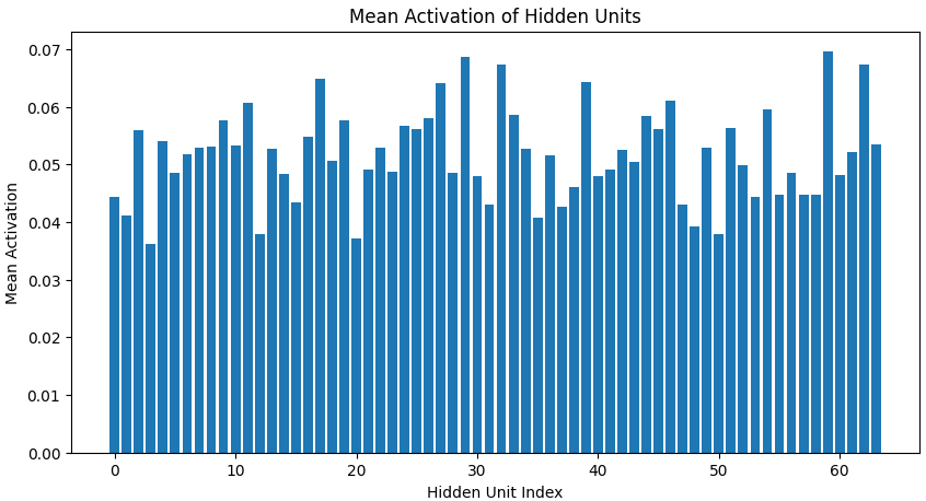
This plot displays the average activation of each hidden neuron in the sparse autoencoder, showing how frequently each unit is used. The lower and uneven activation values indicate that only a few neurons fire strongly while most remain inactive, confirming that the model has learned sparse and specialized feature detectors as intended.
