Introduction to Convolution Neural Network

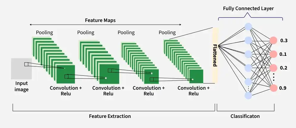
Convolutional Neural Networks (CNNs), are neural network architectures inspired by the human visual system, designed to process image data by capturing spatial relationships between pixels.

• Learn hierarchical features from simple edges to complex objects
• Capture spatial patterns using convolution operations
• Detect objects regardless of their position in the image
• Reduce computation by focusing on local regions instead of the entire image

Key Components of CNN

A complete Convolution Neural Networks architecture is also known as covnets. A covnets is a sequence of layers and every layer transforms one volume to another through a differentiable function. Let’s take an example by running a covnets on of image of dimension 32 x 32 x 3. 

1. Input Layer

The input layer receives the raw image data and passes it to the network for processing. In CNNs, input is typically a 3D volume (width × height × depth).

• Stores pixel values of the image (e.g., 32 × 32 × 3 for RGB images).
• Preserves the spatial structure of the image for further feature extraction.

2. Convolutional Layer

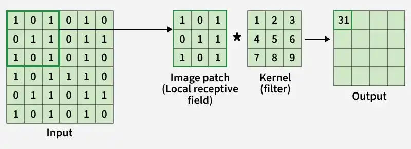
The Convolutional Layer is responsible for extracting important features from the input data. It applies a set of learnable filters (kernels) that slide over the image and compute the dot product between the filter weights and corresponding image patches, producing feature maps.

• Uses small filters (e.g., 2×2, 3×3, 5×5) to scan the input image.
• Generates feature maps that capture patterns such as edges, textures and shapes.

Example: Using 12 filters results in an output volume of 32 × 32 × 12.

3. Activation Layer

The Activation Layer introduces non-linearity into the network by applying an element-wise activation function to the output of the convolution layer. This enables the model to learn complex patterns beyond linear relationships.

• Common activation functions include ReLU, Tanh and Leaky ReLU.
• Applied element-wise to the feature maps.
• The output dimensions remain unchanged (e.g., 32 × 32 × 12).

4. Pooling Layer

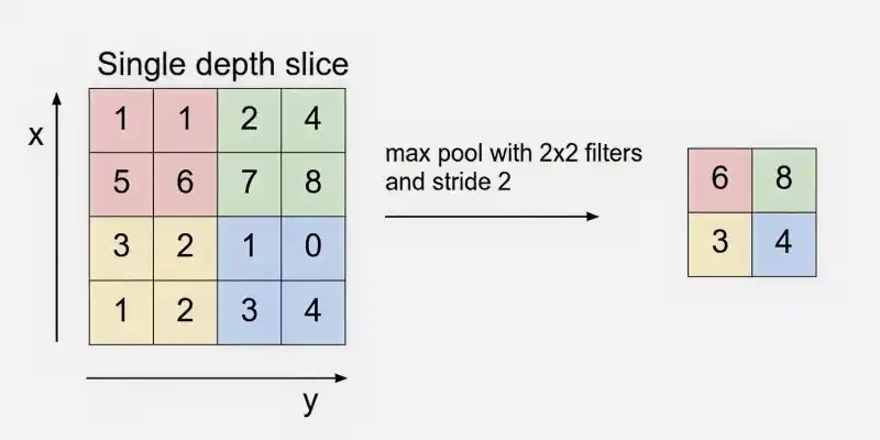
The Pooling Layer is used to reduce the spatial dimensions of the feature maps, making computation faster, reducing memory usage and helping to prevent overfitting. It is typically inserted between convolutional layers in a CNN.

• Common types include Max Pooling and Average Pooling.
• Reduces width and height while keeping depth unchanged.

Example: Using 2 × 2 max pooling with stride 2 reduces the volume from 32 × 32 × 12 to 16 × 16 × 12.

5. Flattening

Flattening converts the multi-dimensional feature maps into a one-dimensional vector after convolution and pooling. This vector is then passed to the fully connected layer for classification or regression.

Example: Flattening 16 × 16 × 12 results in a vector of size 3072 (16 × 16 × 12).

6. Fully Connected Layer

The fully connected (dense) layer performs high-level reasoning using extracted features and produces the final classification scores.

Example: The 3072-length vector is connected to neurons for classification

7. Output Layer

The output layer converts final scores into probabilities using activation functions like Sigmoid (binary classification) or Softmax (multi-class classification).

Example: For 10 classes, Softmax produces 10 probability values each representing the likelihood of a class.

How Convolutional Layers Work

• A small matrix called a filter (kernel) slides over the input image to extract important features.
• At each position, the filter performs element-wise multiplication with the image patch.
• The multiplied values are summed together to produce a single output value.
• This operation is repeated across the entire image using a defined stride.
• The result is a new matrix called a feature map, which highlights detected patterns.
• Multiple filters are applied to capture different features such as edges, textures and shapes.
• The process preserves spatial relationships while reducing the number of learnable parameters compared to fully connected layers.
• Padding can be used to control output size and prevent loss of border information.

Step By Step Implementation

Here we implement a Convolutional Neural Network illustrating how each layer processes and transforms the input image.

Step 1: Import Required Libraries

Here we import TensorFlow for CNN operations and Matplotlib for visualization.

Step 2: Load and Preprocess the Image

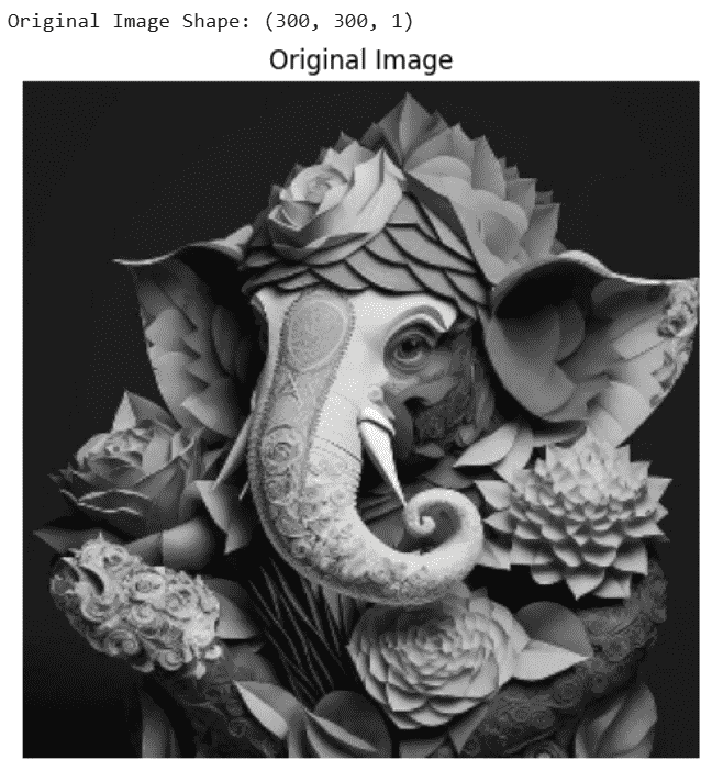
Load the image convert it to grayscale, resize it to 300×300 and normalize pixel values.

Output:

Step 3: Define Convolution Kernel

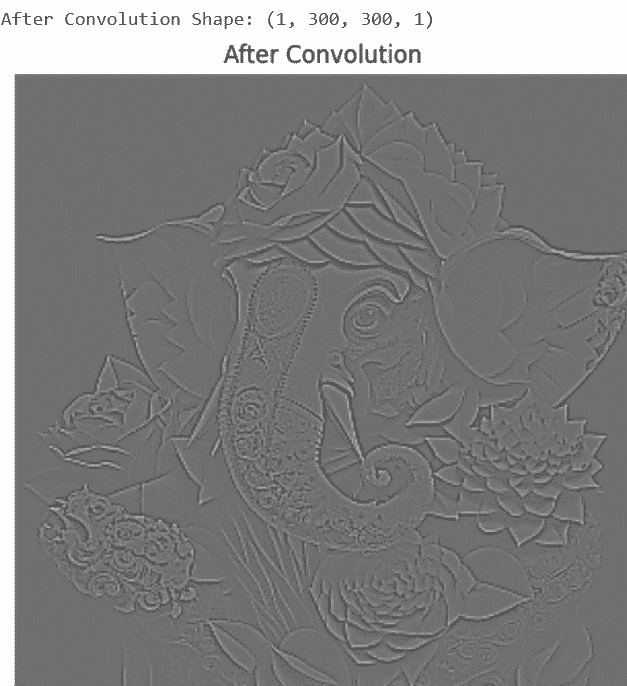
We define an edge detection filter (Laplacian kernel) to extract important image features.

Step 4: Apply Convolution Layer

The convolution layer applies the filter to the image to detect edges and features.

Output:

Step 5: Apply ReLU Activation Function

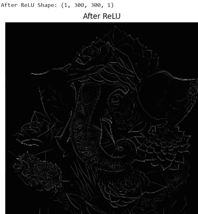
ReLU removes negative values and introduces non-linearity into the network.

Output:

Step 6: Apply Max Pooling Layer

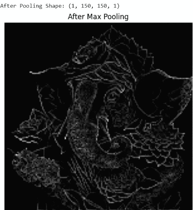
Max pooling reduces spatial dimensions while keeping important features.

Output:

Step 7: Apply Flatten Layer

The flatten layer converts 2D feature maps into a 1D feature vector for fully connected layers.

Output:

After Flatten Shape: (1, 22500)

First 20 values of Flattened Vector:

[135. 81. 81. 81. 81. 81. 81. 81. 81. 81. 81. 81. 81. 81.

81. 81. 81. 81. 81. 81.]

Step 8: Add Fully Connected (Dense) Layer

The fully connected layer learns high-level patterns from the flattened feature vector and produces output predictions.

Output:

After Fully Connected Layer Shape: (1, 64)

You can download full code from here

Advantages

• Automatically learn important features from images, videos or audio without manual extraction.
• Highly effective at detecting spatial patterns, edges, textures and shapes.
• Robust to variations like translation, rotation and scaling in input data.
• Can handle large datasets and achieve high predictive accuracy.
• Supports end-to-end training, simplifying the model pipeline.

Limitations

• Training is computationally intensive and requires significant memory.
• Prone to overfitting if data is limited or regularization is insufficient.
• Requires large amounts of labeled data for optimal performance.
• Limited interpretability difficult to understand learned features.
• Sensitive to adversarial examples and noise in input data.