Architecture and Learning process in neural network

Neural networks are a core part of machine learning that learn patterns from data to make predictions. Inspired by the human brain, they use interconnected neurons arranged in layers to process information efficiently.

• Inspired by the structure of the human brain
• Made up of interconnected artificial neurons
• Organized into input, hidden and output layers
• Learn patterns from data through training
• Used for tasks like prediction, classification and pattern recognition

Architectures of Neural Network

Neural network architecture defines how neurons are arranged and connected to process data and learn patterns. It uses multiple layers where data flows forward through weighted connections and activation functions to produce outputs.

• Consists of input, hidden, and output layers, each handling a stage of data processing
• Neurons are connected through weights that control the flow of information
• Hidden layers perform intermediate computations to learn complex patterns
• Activation functions like ReLU, sigmoid, and softmax introduce non-linearity
• The choice of layers and neurons affects accuracy, speed, and performance

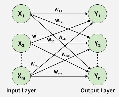
1. Single-layer Feed Forward Network

A single-layer feed forward network is the simplest type of neural network where data moves directly from input to output without any hidden layers. It is suitable for simple, linearly separable problems.

• Has only an input layer and an output layer
• Inputs are passed through weighted connections to the output
• The output neuron computes a weighted sum and applies an activation function
• Model learns by updating weights using backpropagation
• Easy to implement but cannot handle complex non-linear relationships

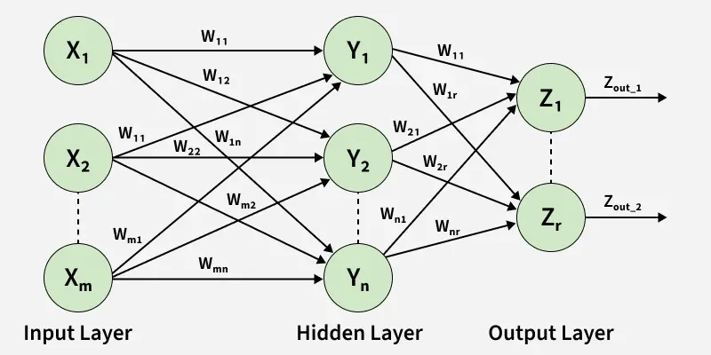
2. Multi-layer Feed Forward Network

A multi-layer feed forward network extends basic neural networks by adding one or more hidden layers between input and output, allowing it to learn complex non-linear patterns.

• Contains input, multiple hidden layers and an output layer
• Processes input data through successive layers to generate predictions
• Hidden layers learn higher-level representations using weights and activation functions
• Learns by updating weights through backpropagation
• Effective for complex tasks like image recognition, speech processing and NLP

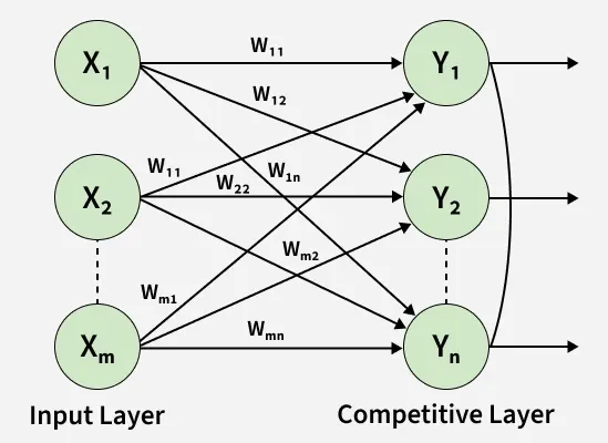
3. Competitive Network

A competitive network is a type of neural network where output neurons compete with each other to respond to an input. It uses unsupervised learning to discover patterns and group similar data.

• Output neurons compete, and only one (or a few) becomes active (winner-takes-all)
• Uses unsupervised learning to find patterns without labeled data
• The winning neuron updates its weights to match the input better
• Helps organize data into clusters or groups over time
• Activation is based on similarity or distance, and non-winning neurons are suppressed

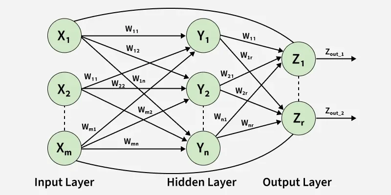
4. Recurrent Network

A recurrent neural network is designed to work with sequential data by using feedback connections, allowing it to remember past information and model time-based patterns.

• Uses feedback loops so previous outputs influence current predictions
• Maintains an internal state to capture sequence context
• Suitable for tasks like time-series prediction, speech recognition and NLP
• Trained using Backpropagation Through Time (BPTT) to update weights across time steps

Learning Process in Artificial Neural Networks

The learning process in an Artificial Neural Network involves training the model to learn patterns from data by adjusting its parameters to reduce error and improve accuracy.

1. Number of Layers in the Network

The number of layers in a neural network determines its ability to learn patterns, ranging from simple to complex relationships in data.

• Single-layer networks have only input and output layers and are suitable for simple, linearly separable problems
• Multi-layer networks include hidden layers that help learn complex and non-linear patterns

2. Direction of Signal Flow

The direction of signal flow defines how information moves through the network and how past information is used.

• Feedforward networks pass data only from input to output
• Recurrent networks use feedback connections to capture sequence and time-based information

3. Number of Nodes in Layers

The number of nodes in each layer determines the network’s capacity to learn and represent data.

• Input nodes represent features, and output nodes represent target classes
• Hidden nodes are user-defined and control learning capability
• Too many nodes can cause overfitting and increase computational cost

4. Weights of Interconnected Nodes

Weights define the strength of connections between neurons and are key to the learning process.

• Represent how strongly one neuron influences another
• Initialized randomly and updated during training
• Adjusted iteratively until error is minimized or a stopping condition is reached

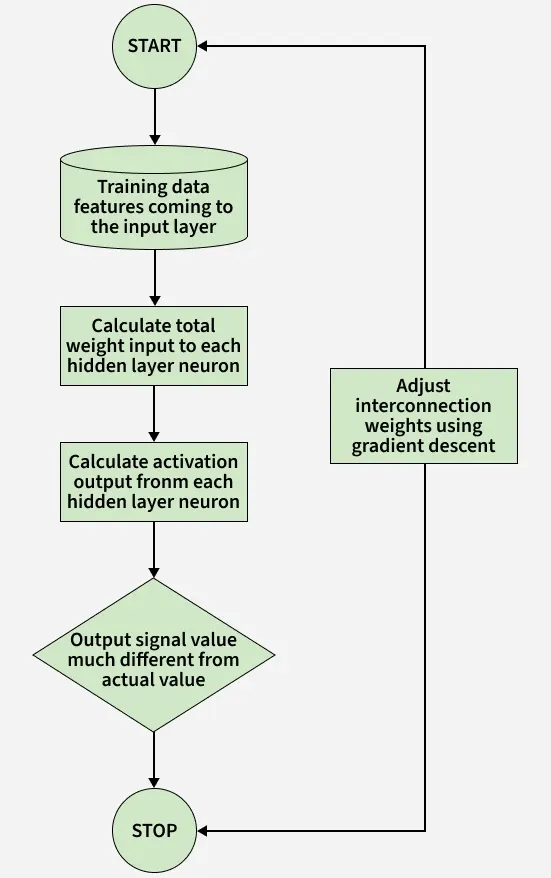
Backpropagation in ANN

Backpropagation is a learning process in neural networks that reduces prediction error by updating weights based on the difference between actual and predicted outputs. It uses gradient descent to optimize these weights efficiently.

• Calculates the error between predicted output and target output
• Propagates this error backward through the network
• Updates weights to reduce the error
• Repeats iteratively to improve model accuracy over time

Phases of Backpropagation

Backpropagation works in two main phases to train a neural network by first generating outputs and then correcting errors.

1. Forward Phase

In the forward phase the input signals propagate from the input layer to the output layer through one or more hidden layers. During this process

• Weighted sums of inputs are calculated at each neuron.
• Activation functions are applied to generate neuron outputs.
• The final output of the network is obtained at the output layer.

2. Backward Phase

In this phase, the error is calculated and propagated backward to update weights.

• The network output is compared with the expected output.
• The error is calculated at the output layer.
• This error is propagated backward through the network.
• The propagated error is used to adjust the interconnection weights to reduce the overall error.

Multi-Layer Feedforward Neural Network

Let's Consider a multi-layer feedforward neural network

1. Hidden Layer Computation

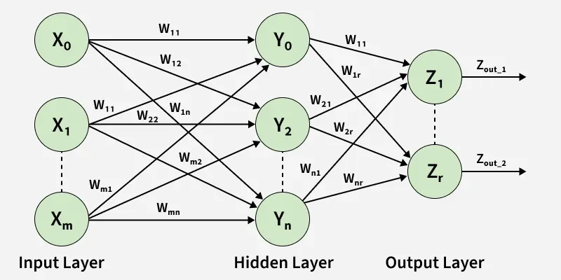
The net input to the k-th hidden neuron is given by

Here denotes the bias input

The output of the k-th hidden neuron is obtained by applying the hidden layer activation function to the net input:

where

• : Net input to the k-th hidden neuron
• : Output of the k-th hidden neuron after activation
• : Weight connecting the i-th input neuron to the k-th hidden neuron
• m: Total number of input features

2. Output Layer Computation

The net input to the k-th output neuron is obtained by summing the weighted outputs of all hidden layer neurons and adding a bias term. The bias input allows the model to shift the activation function and improves learning flexibility.

where

• is Net input to the k-th output neuron
• is the weight connecting the i-th hidden neuron to the k-th output neuron
• is the number of hidden neurons.

The final output of the output neuron

This step produces the network’s predicted output for the given input

3. Error (Cost) Function

Let be the target output of the output neuron. The cost function defined as the sum of squared errors is:

Since the output neuron applies an activation function the error can also be written as:

4. Weight Update for Hidden-to-Output Layer

To update the weights using gradient descent, the partial derivative of the error with respect to the weight (connecting hidden neuron to output neuron ) is computed as:

5. Weight and Bias Update Equations

Using learning rate the weight update rule is:

For the bias weight:

6. Weight Update for Input-to-Hidden Layer

The weights connecting the input layer to the hidden layer are updated using the gradient descent method. To determine how each weight should be changed, we compute the gradient of the error function with respect to the weight using the chain rule.

For weights change in weight is given by:

Using the chain rule this gradient can be expanded as:

weight update:

Applications

• Used for tasks like face recognition and object detection
• Applied in NLP for text classification, translation and chatbots
• Enables speech recognition and voice-controlled systems
• Helps in disease detection and medical image analysis
• Supports fraud detection and credit scoring in finance

Advantages

• Can handle complex tasks like image processing and natural language processing
• Learns non-linear relationships from data effectively
• Automatically extracts important features from raw data
• Achieves high accuracy with large datasets
• Performs well even with noisy or incomplete data

Limitations

• Require a large amount of training data to perform well
• Need high computational power and longer training time
• Act as a black-box, making decisions hard to interpret
• Can overfit when data is limited or noisy
• Require careful tuning of layers, parameters and hyperparameters