How to implement cost-sensitive learning in decision trees?

Decision trees are tools for classification, but they can struggle with imbalanced datasets where one class significantly outnumbers the other. Cost-sensitive learning is a technique that addresses this issue by assigning different costs to misclassification errors, making the decision tree more sensitive to the minority class. Cost-sensitive learning is implemented in decision trees by using weighted splits, alternative splitting criteria, and adjusting the class weights.

Decision Trees can be utilized for cost- sensitive learning by adjusting the weights related to each of the classes.

Understanding Cost-Sensitive Learning

Cost-sensitive learning is a type of learning that takes into account the misclassification costs, which can be different for each class. This approach is particularly useful in imbalanced classification problems where the cost of misclassifying a minority class instance is often higher than that of the majority class.

Using Class Weights

One of the most common methods to implement cost-sensitive learning in decision trees is by using class weights. This involves assigning higher weights to instances from the minority class, making the tree more sensitive to these instances.

Heuristics for Setting Class Weights

1. Inverse Class Distribution: A common heuristic is to use the inverse of the class distribution present in the training dataset. For instance, if the class distribution is 1:100 for the minority to majority class, you can use weights of 1 for the majority class and 100 for the minority class.

2. Domain Expertise and Tuning: Class weights can also be determined through domain expertise or by performing a hyperparameter search using techniques like grid search. This allows you to find the optimal weights that result in the best performance.

Alternative Splitting Criteria

Cost Matrix: Instead of using the default Gini index or entropy, you can use a cost matrix to define the misclassification costs.

Implementing Weight Balancing with Decision Trees

Creating/Importing an imbalanced dataset:

Output:

Class distribution: Counter({np.int64(0): 990, np.int64(1): 10})

In this Code we create an imbalanced dataset for our example using the make_classification module. Now we train and plot different

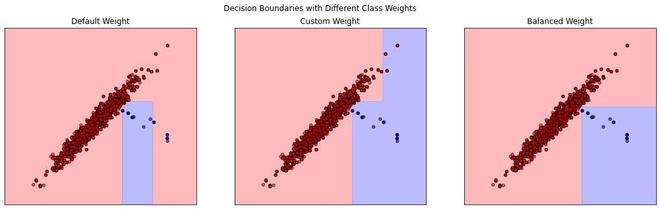
Now we now train a `DecisionTreeClassifier` on it with three different class weight configurations: default, custom (`{0: 1, 1: 5}`), and balanced. Each configuration is visualized by plotting the decision boundaries, showing how different class weights affect the classifier's decision regions. Additionally, a classification report and ROC AUC score for each configuration are printed to assess performance.

Output:

Class report with Default Weight:
 precision recall f1-score support

 0 1.00 1.00 1.00 990
 1 0.75 0.60 0.67 10

 accuracy 0.99 1000
 macro avg 0.87 0.80 0.83 1000
weighted avg 0.99 0.99 0.99 1000

Class report with Custom Weight:
 precision recall f1-score support

 0 1.00 0.99 1.00 990
 1 0.67 1.00 0.80 10

 accuracy 0.99 1000
 macro avg 0.83 1.00 0.90 1000
weighted avg 1.00 0.99 1.00 1000

Class report with Balanced Weight:
 precision recall f1-score support

 0 1.00 1.00 1.00 990
 1 1.00 1.00 1.00 10

 accuracy 1.00 1000
 macro avg 1.00 1.00 1.00 1000
weighted avg 1.00 1.00 1.00 1000

We can visualize this better using the decision boundaries.

Key Takeaways on How to implement cost-sensitive learning in decision trees

• Class Weights: Assign higher weights to the minority class to make the decision tree more sensitive to these instances.
• Heuristics: Use the inverse of the class distribution or domain expertise to set the class weights.
• Alternative Splitting Criteria: Use a cost matrix to define different misclassification costs.
• Hyperparameter Tuning: Perform grid search or other hyperparameter tuning methods to find the optimal class weights.