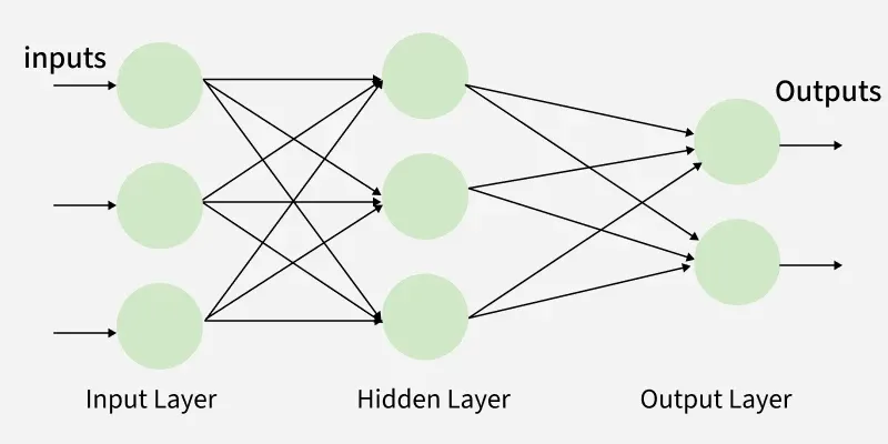
Multi-Layer Perceptron Learning in Tensorflow

Multi-Layer Perceptron (MLP) consists of fully connected dense layers that transform input data from one dimension to another. It is called multi-layer because it contains an input layer, one or more hidden layers and an output layer. The purpose of an MLP is to model complex relationships between inputs and outputs.

Components of MLP

• Input Layer: Each neuron or node in this layer corresponds to an input feature. For instance, if you have three input features the input layer will have three neurons.
• Hidden Layers: MLP can have any number of hidden layers with each layer containing any number of nodes. These layers process the information received from the input layer.
• Output Layer: The output layer generates the final prediction or result. If there are multiple outputs, the output layer will have a corresponding number of neurons.

Working of Multi-Layer Perceptron

Let's see working of the multi-layer perceptron. The key mechanisms such as forward propagation, loss function, backpropagation and optimization.

1. Forward Propagation

In forward propagation the data flows from the input layer to the output layer, passing through any hidden layers. Each neuron in the hidden layers processes the input as follows:

Weighted Sum: The neuron computes the weighted sum of the inputs:

Where:

• ​ is the input feature.
• ​ is the corresponding weight.
• is the bias term.

Activation Function: The weighted sum z is passed through an activation function to introduce non-linearity. Common activation functions include:

• Sigmoid:
• ReLU (Rectified Linear Unit):
• Tanh (Hyperbolic Tangent):

2. Loss Function

Once the network generates an output the next step is to calculate the loss using a loss function. In supervised learning this compares the predicted output to the actual label.

For a classification problem the commonly used binary cross-entropy loss function is:

Where:

• is the actual label.
• is the predicted label.
• is the number of samples.

For regression problems the mean squared error (MSE) is often used:

3. Backpropagation

The goal of training an MLP is to minimize the loss function by adjusting the network's weights and biases. This is achieved through backpropagation:

1. Gradient Calculation: The gradients of the loss function with respect to each weight and bias are calculated using the chain rule of calculus.
2. Error Propagation: The error is propagated back through the network, layer by layer.
3. Gradient Descent: The network updates the weights and biases by moving in the opposite direction of the gradient to reduce the loss:

Where:

• is the weight.
• is the learning rate.
• is the gradient of the loss function with respect to the weight.

4. Optimization

MLPs rely on optimization algorithms to iteratively refine the weights and biases during training. Popular optimization methods include:

• Stochastic Gradient Descent (SGD): Updates the weights based on a single sample or a small batch of data:
• Adam Optimizer: An extension of SGD that incorporates momentum and adaptive learning rates for more efficient training:

Here ​ represents the gradient at time and are decay rates.

Now that we are done with the theory part of multi-layer perception, let's go ahead and implement code in python using the TensorFlow library.

Implementing Multi Layer Perceptron

1. Importing Modules and Loading Dataset

First we import necessary libraries such as TensorFlow, NumPy and Matplotlib for visualizing the data. We also load the MNIST dataset.

2. Loading and Normalizing Image Data

Next we normalize the image data by dividing by 255 (since pixel values range from 0 to 255) which helps in faster convergence during training.

Output:

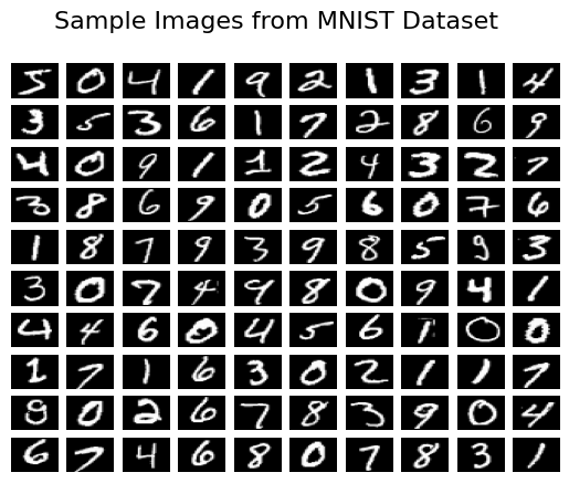
3. Visualizing Data

To understand the data better we plot the first 100 training samples each representing a digit.

Output:

4. Building the Neural Network Model

A Sequential neural network model is created with the following layers:

• Flatten Layer: Converts the 28×28 pixel image into a one-dimensional array of 784 values.
• Hidden Layers: Two fully connected (Dense) layers with 256 and 128 neurons, using the sigmoid activation function.
• Output Layer: A Dense layer with 10 neurons representing the digit classes (0–9), using the softmax activation function to produce class probabilities.

5. Compiling the Model

Once the model is defined we compile it by specifying:

• Optimizer: Adam for efficient weight updates.
• Loss Function: Sparse categorical cross entropy, which is suitable for multi-class classification.
• Metrics: Accuracy to evaluate model performance.

6. Training the Model

We train the model on the training data using 10 epochs and a batch size of 2000. We also use 20% of the training data for validation to monitor the model’s performance on unseen data during training.

Output:

7. Evaluating the Model

After training we evaluate the model on the test dataset to determine its performance.

Output:

Test loss, Test accuracy: [0.2682029604911804, 0.9257000088691711]

We got the accuracy of our model 92% by using model.evaluate() on the test samples.

8. Visualizing Training and Validation Loss VS Accuracy

Output:

The model is learning effectively on the training set, but the validation accuracy and loss levels off which might indicate that the model is starting to overfit.

Advantages

• Versatility: MLPs can be applied to a variety of problems, both classification and regression.
• Non-linearity: Using activation functions MLPs can model complex, non-linear relationships in data.
• Parallel Computation: With the help of GPUs, MLPs can be trained quickly by takfing advantage of parallel computing.

Limitations

• Computationally Expensive: MLPs can be slow to train especially on large datasets with many layers.
• Prone to Overfitting: Without proper regularization techniques they can overfit the training data leading to poor generalization.
• Sensitivity to Data Scaling: They require properly normalized or scaled data for optimal performance.