Machine Learning Model Evaluation

Model evaluation is the process of assessing how well a machine learning model performs on unseen data using different metrics and techniques. It ensures that the model not only memorises training data but also generalises to new situations. By applying various techniques, we can identify whether a model has truly learned patterns or not.

1. Cross-Validation

Cross-validation ensures that the model is tested on multiple subsets of data making it less likely to overfit and improving its generalisation ability.

(a) Holdout Method

In the Holdout method the dataset is split into train and test sets (commonly 7:3 or 8:2). Let's implement it where:

• load_iris() loads the Iris dataset (flower measurements with 3 species).
• train_test_split() divides data into training and testing sets.
• test_size=0.20: 20% for testing, 80% for training.
• random_state=42 makes results reproducible

Output:

Training set size: 120
Testing set size: 30

(b) K-Fold Cross-Validation

In K-Fold Cross-Validation the dataset is divided into k folds. Each fold is used once as a test set and the model is trained on the remaining k-1 folds. Lets implement it where:

• DecisionTreeClassifier(): A decision tree model is created.
• KFold(n_splits=5): Data is divided into 5 folds.
• cross_val_score(): Runs training/testing across folds.
• scores: Accuracy for each fold.
• scores.mean(): Average accuracy across all folds.

Output:

Cross-validation scores: [1. 1. 0.93333333 0.93333333 0.93333333]
Average CV Score: 0.9600000000000002

2. Evaluation Metrics for Classification Tasks

Classification models assign inputs to predefined labels. Their performance can be measured using accuracy, precision, recall, F1 score, confusion matrix and AUC-ROC. We’ll demonstrate these metrics using a Decision Tree Classifier on the Iris dataset.

Step 1: Importing Libraries, Loading Dataset, Splitting Dataset

• Importing libraries like pandas, numpy, matplotlib and scikit learn.
• Loading Iris dataset with flower measurements.
• Splitting into 80% training, 20% testing.

Step 2: Training Model

• DecisionTreeClassifier(): Creates a decision tree model.
• .fit(X_train, y_train): Trains the model on training data.
• .predict(X_test): Generates predictions on test data.

Step 3: Accuracy

We will calculate the accuracy,

• TP: True Positives
• TN: True Negatives
• FP: False Positives
• FN: False Negatives

accuracy_score() computes the proportion of correct predictions.

Output:

Accuracy: 0.9333333333333333

Step 4: Precision and Recall

Precision: Precision measures how many predicted positives are actually positive.

• Focuses on the correctness of positive predictions.
• High precision: few false positives.

Recall: Recall measures how many actual positives are correctly predicted.

• Focuses on capturing all positives.
• High recall: few false negatives.

Output:

Precision: 0.9435897435897436
Recall: 0.9333333333333333

For more details regarding Precision and Recall please refer to: Precision and Recall in Machine Learning

Step 5: F1 Score

We will calculate the F1 score which is Harmonic mean of precision and recall. Balances both metrics.

• Combines precision and recall into one metric.
• Useful when we need a balance between false positives and false negatives.

Output:

F1 score: 0.9327777777777778

Step 6: Confusion Matrix

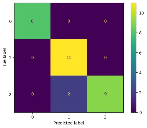
We will create a confusion matrix:

• confusion_matrix(): Creates matrix of actual vs predicted values.
• Each cell shows correct/misclassified predictions.

Output:

Step 7: AUC-ROC Curve

AUC -ROC Curve measures the area under the ROC curve, indicating the model’s ability to distinguish classes.

• TPR: True Positive Rate
• FPR: False Positive Rate
• AUC: Area under curve; higher is better (0.5 random, 1 perfect).

Output:

AUC: 0.9473684210526316

3. Evaluation Metrics for Regression Tasks

Regression predicts continuous values (e.g., temperature). We use error-based metrics to measure accuracy.

We will use the weather dataset which can be downloaded from here.

Step 1: Importing Data and Training Model

• Dataset contains Temperature (independent variable) and Relative Humidity (dependent variable).
• Data split into training (80%) and testing (20%).
• LinearRegression().fit() trains the regression model.
• Predictions are stored in Y_pred.

Step 2: Mean Absolute Error (MAE)

Mean absolute error is average difference between actual and predicted values.

• : Actual value
• ​: Predicted value
• : Number of samples

Output:

MAE: 2.2349999999999977

Step 3: Mean Squared Error (MSE)

We will calculate the mean squared error which is average squared difference between predicted and actual values.

• Penalizes larger errors more than MAE.
• Commonly used for regression model loss functions.

Output:

MSE: 6.470558999999991

Step 4: Root Mean Squared Error (RMSE)

We will calculate RMSE which is Square root of MSE. Converts error back to original units.

• Brings error back to the same units as the target variable.
• Easier to interpret than MSE.
• Still penalizes larger errors more than MAE.

Output:

RMSE: 2.54372934881052

Step 5: Mean Absolute Percentage Error (MAPE)

MAPE expresses the prediction error as a percentage of the actual value.

• Tells us how “off” predictions are in percentage terms.
• Useful for business metrics (e.g., sales forecast error).
• Sensitive when actual values are very small (can blow up).

Output:

MAPE: 0.03925255003024494