Data Visualization with Seaborn - Python

Seaborn is a Python library for creating attractive statistical visualizations. Built on Matplotlib and integrated with Pandas, it simplifies complex plots like line charts, heatmaps and violin plots with minimal code.

Creating Plots with Seaborn

Seaborn makes it easy to create clear and informative statistical plots with just a few lines of code. It offers built-in themes, color palettes, and functions tailored for different types of data.

Let’s see various types of plots with simple code to understand how to use it effectively.

1. Line plot

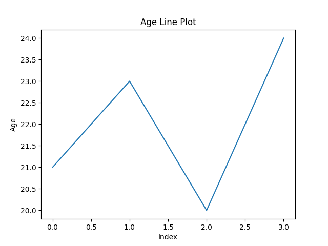
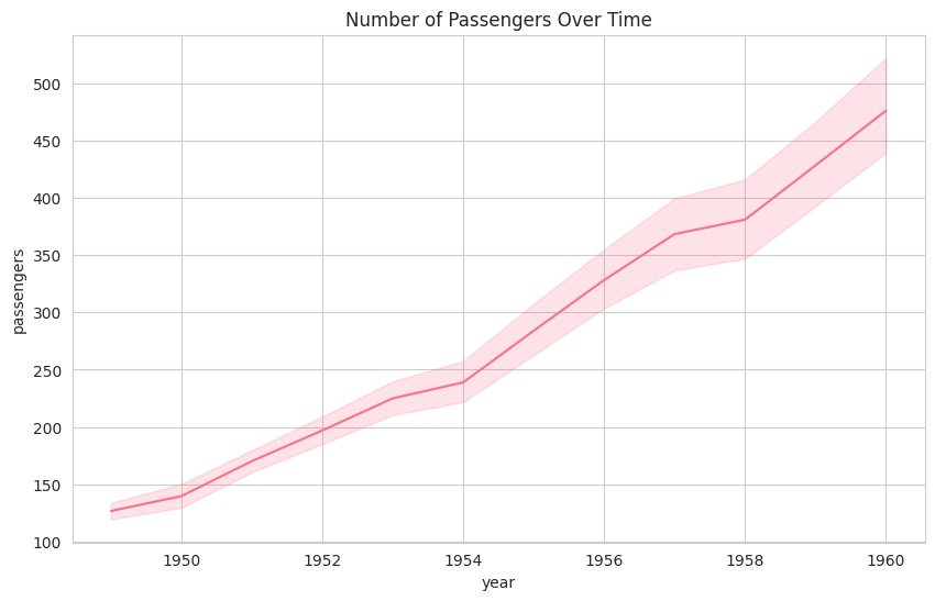
A line plot shows the relationship between two numeric variables, often over time. It can also compare multiple groups using different lines.

Syntax:

sns.lineplot(x=None, y=None, data=None)

Parameters:

• x, y: Numeric input variables. These can be arrays, lists or column names from a DataFrame.
• data: DataFrame containing the data.

Example:

Output

2. Scatter Plot

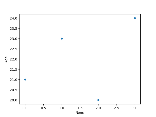
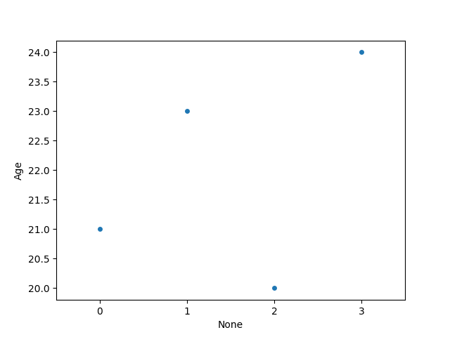
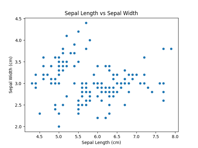
Scatter plots are used to visualize the relationship between two numerical variables. They help identify correlations or patterns. It can draw a two-dimensional graph.

Syntax:

sns.scatterplot(x=None, y=None, data=None)

Parameters:

• x, y: Input data variables that should be numeric.
• data (optional): Dataset containing the variables.

Returns: An Axes object with the scatter plot.

Example:

Output

3. Box plot

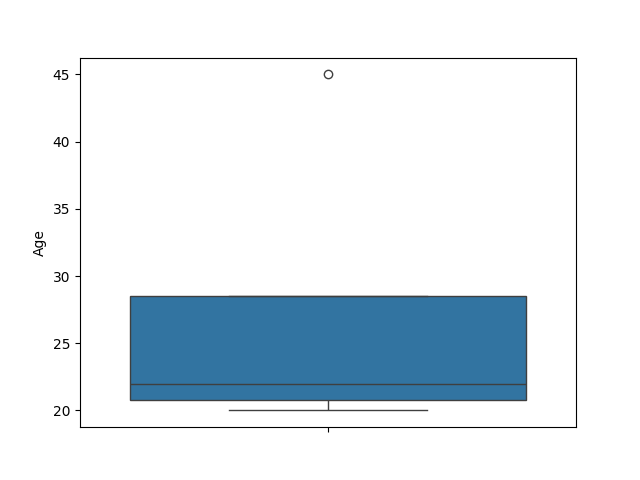
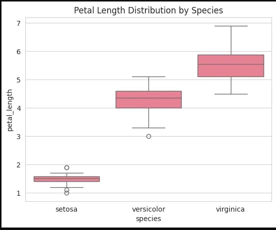
A box plot is the visual representation of the depicting groups of numerical data with their quartiles against continuous/categorical data.

It consists of 5 key statistics: Minimum ,First Quartile or 25% , Median (Second Quartile) or 50%, Third Quartile or 75% and Maximum

Syntax:

sns.boxplot(x=None, y=None, hue=None, data=None)

Parameters:

• x, y, hue: Variables for plotting long-form data.
• data: Dataset to plot. If x and y are absent data is treated as wide-form.

Returns: An Axes object with the box plot.

Example:

Output

4. Violin Plot

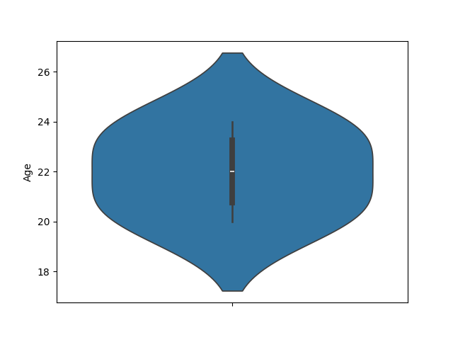
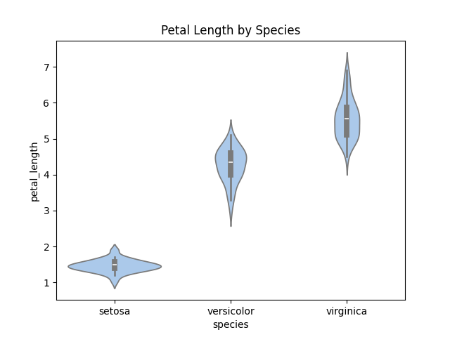
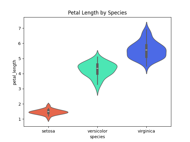
A violin plot is similar to a boxplot. It shows several quantitative data across one or more categorical variables such that those distributions can be compared.

Syntax:

sns.violinplot(x=None, y=None, hue=None, data=None)

Parameters: 

• x, y, hue: Inputs for plotting long-form data. 
• data: Dataset for plotting. 

Example:

Output

5. Swarm plot

A swarm plot displays individual data points without overlap along a categorical axis which provides a clear view of distribution density.

Syntax:

sns.swarmplot(x=None, y=None, hue=None, data=None)

Parameters: 

• x, y, hue: Inputs for plotting long-form data. 
• data: Dataset for plotting. 

Example:

Output

6. Bar plot

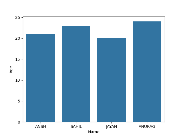
Barplot represents an estimate of central tendency for a numeric variable with the height of each rectangle and provides some indication of the uncertainty around that estimate using error bars. 

Syntax:

sns.barplot(x=None, y=None, hue=None, data=None)

Parameters :

• x, y : Variables or column names for long-form data.
• hue : (optional) Column for color encoding.
• data : (optional) Dataset to plot.

Returns: Axes object with the bar plot.

Example:

Output

7. Point plot

Point plot show point estimates and confidence intervals using scatter glyphs which represents the central tendency of a numeric variable.

Syntax:

sns.pointplot(x=None, y=None, hue=None, data=None)

Parameters:

• x, y: Inputs for plotting long-form data.
• hue: (optional) column name for color encoding.
• data: Dataframe as a Dataset for plotting.

Return: Axes object with the point plot.

Example:

Output

8. Count plot

A Count plot displays the number of occurrences of each category using bars to visualize the distribution of categorical variables.

Syntax :

sns.countplot(x=None, y=None, hue=None, data=None)

Parameters :

• x, y: Inputs for plotting long-form data.
• hue: (optional) column name for color encoding.
• data: Dataframe as a Dataset for plotting.

Returns: Axes object with the count plot.

Example:

Output

9. KDE Plot

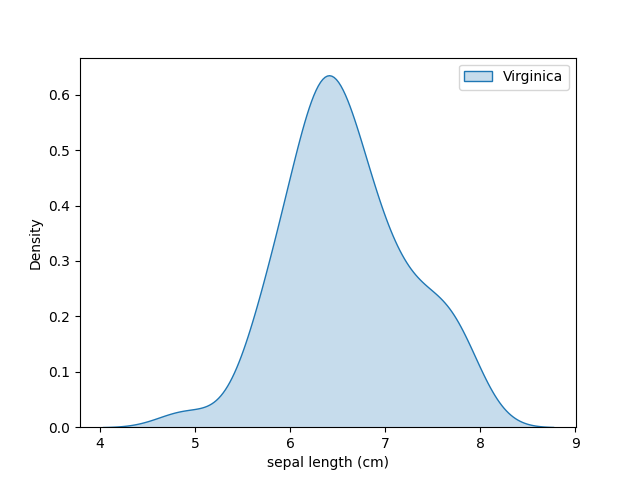
KDE Plot (Kernel Density Estimate) is used for visualizing the Probability Density of a continuous variable at different values in a continuous variable. We can also plot a single graph for multiple samples which helps in more efficient data visualization.

Syntax:

sns.kdeplot(data=None, x=None, y=None, fill=False)

Parameters:

• x, y: Vectors or data keys.
• vertical: Boolean to plot vertically.
• palette: Color palette.
• data: Dataframe

Example:

Output

How to Customize Seaborn Plots with Python?

Customizing Seaborn plots increases their readability and visual appeal which makes the data insights clearer and more informative. Here are several ways we can customize our plots in Seaborn:

1. Adding Titles and Axis Labels

Adding descriptive titles and axis labels makes our plots more understandable and informative. Using Matplotlib's plt.title(), plt.xlabel() and plt.ylabel() to set titles and axis labels.

Output

2. Built-in Styles and Grids in Seaborn

Seaborn provides built-in styles that control the background and grid of your plots. These styles improve readability and can be chosen based on your presentation needs.

Available Styles:

• darkgrid – Dark background with light gridlines. Great for clear contrast.
• whitegrid – White background with light gridlines. Ideal for statistical plots.
• dark – Dark background without gridlines. Clean and modern look.
• white – Plain white background without gridlines. Good for simple visuals.
• ticks – White background with axis ticks styled sharply. Suitable for publications.

Output

3. Customizing Color Palettes

Seaborn makes it easy to enhance the appearance of plots using color palettes. You can choose from built-in palettes like "deep", "muted", or "bright" or define your own using sns.color_palette(). Customizing colors improves clarity and helps match your data’s theme or purpose.

a) Using a Built-in Palette:

Output

b) Using a Custom Palette:

4. Adjusting Figure Size and Aspect Ratio

We can adjust the figure size using plt.figure(figsize=(width,height)) to control the plot's dimensions. This allows for better customization to fit different presentation or reports.

Output

5. Adding Markers to Line Plots

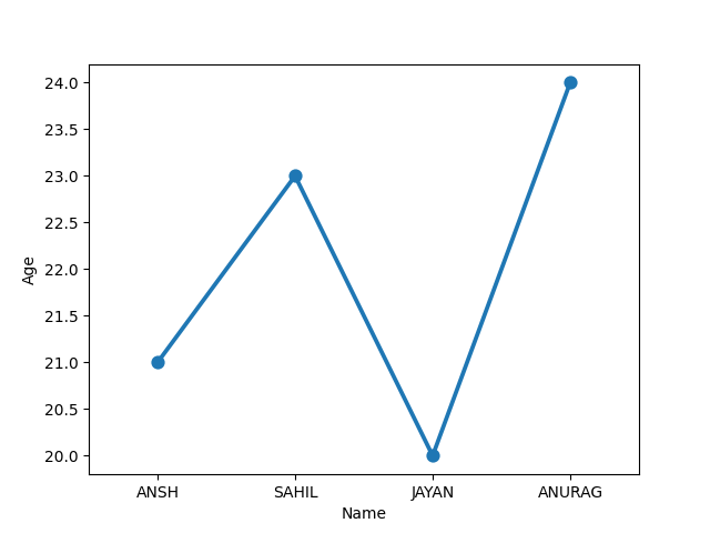
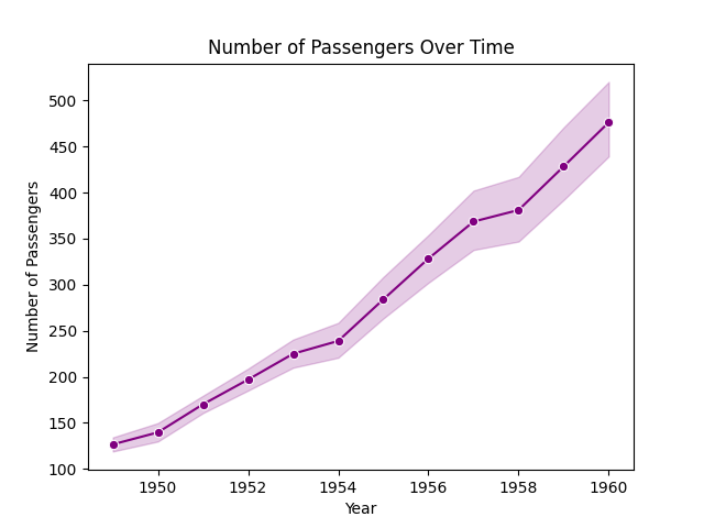
Markers can be added to Seaborn line plots using the marker argument to highlight data points. For example adding circular markers to the line plot using sns.lineplot(x='x', y='y' ,marker='o')

Output

Visualizing Relationships and Patterns with Seaborn

We’ll see various plots in Seaborn for visualizing relationships, distributions and trends across our dataset. These visualizations help to find hidden patterns and correlations in datasets with multiple variables.

1. Pair Plots

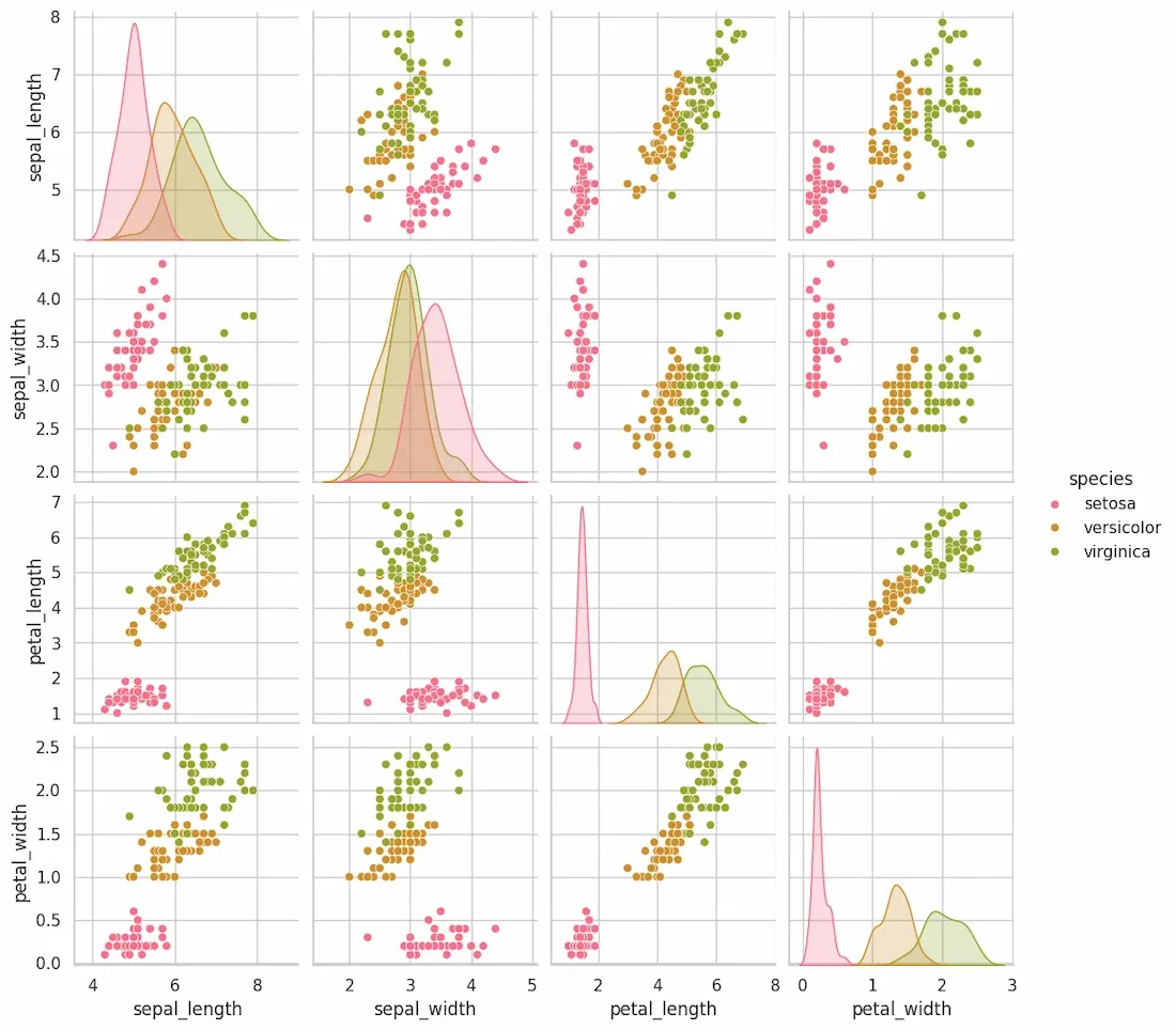
Pair plots are used explore relationships between several variables by generating scatter plots for every pair of variables in a dataset along with univariate distributions on the diagonal. This is useful for exploring datasets with multiple variables and seeing potential correlations.

Syntax:

sns.pairplot(data, hue=None)

Parameters:

• data: Dataset to plot.
• hue: (optional) Categorical variable used for color coding data points.

Returns: An array of Axes objects containing the scatter plot grid and distributions.

Example:

Output

2. Joint Plots

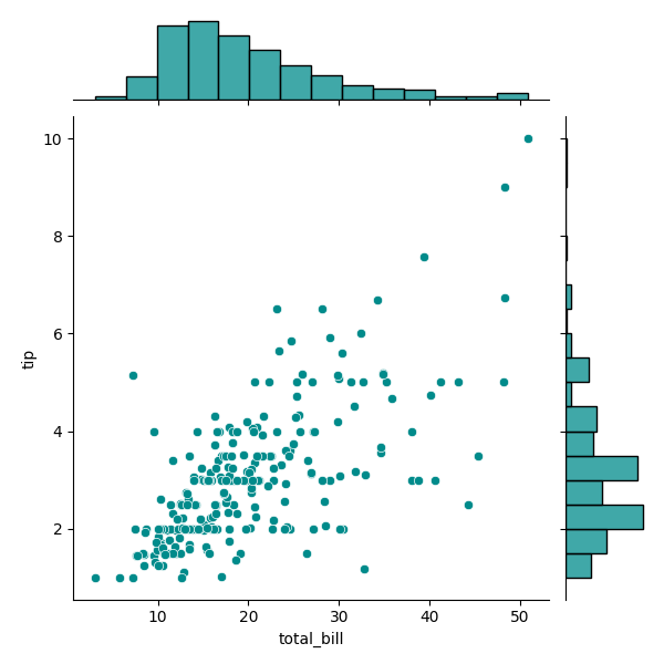
Joint plots combine a scatter plot with the distributions of the individual variables. This allows for a quick visual representation of how the variables are distributed individually and how they relate to one another.

Syntax:

sns.jointplot(x, y, data, kind='scatter')

Parameters:

• x, y: Variables to plot.
• data: Dataset to plot.
• kind: Type of plot to display ('scatter', 'kde', 'reg' etc).

Returns:

An Axes object with the joint plot including scatter plot and distribution plots on the margins.

Example:

Output

This creates a scatter plot between total_bill and tip with histograms of the individual distributions along the margins. The kind parameter can be set to 'kde' for kernel density estimates or 'reg' for regression plots.

3. Grid Plot

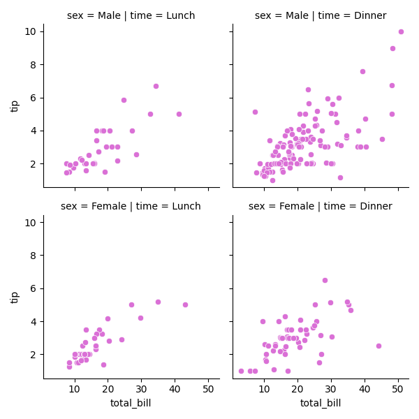
Grid plots in Seaborn are used to create multiple subplots in a grid layout. Using Seaborn's FacetGrid we can visualize how variables interact across different categories which makes it easier to compare groups or conditions within our dataset.

Syntax:

g = sns.FacetGrid(data, col='column_name', row='row_name')
g.map(sns.scatterplot, 'x', 'y')

Parameters:

• data: Dataset to plot.
• col, row: Variables for the columns and rows of the grid (categorical variables).
• sns.scatterplot: The plotting function to apply to each facet.

Returns: A FacetGrid object with the grid of plots.

Example: To use FacetGrid, we first need to initialize it with a dataset and specify the variables that will form the row, column or hue dimensions of the grid. Here is an example using the tips dataset:

Output

Regression Plots: Visualizing Linear Relationships

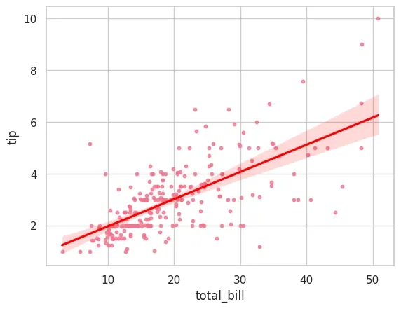
Seaborn simplifies the process of performing and visualizing regressions specifically linear regressions which is important for identifying relationships between variables, detecting trends and making predictions. It supports two primary functions for regression visualization:

• regplot(): This function plots a scatter plot along with a linear regression model fit.
• lmplot(): This function also plots linear models but provides more flexibility in handling multiple facets and datasets.

Example: Let’s use a simple dataset to visualize a linear regression between two variables: x (independent variable) and y (dependent variable).

Output:

As we explore Seaborn functions and techniques we can create clear, customized and insightful visualizations that helps us to understand our data better.