Image classification is a fundamental task in computer vision where a model learns to identify and assign labels to images based on their visual content. It plays a key role in applications such as object recognition, facial detection, and autonomous systems. CIFAR‑10 image classification is a popular computer vision task that involves training models to recognize objects across ten distinct categories using the CIFAR‑10 dataset.
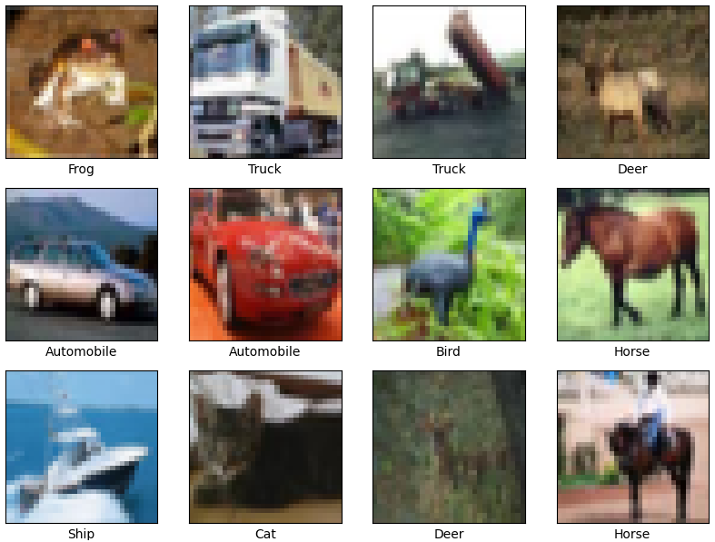
Uses a standard benchmark dataset with 60,000 labelled images Commonly implemented with convolutional neural networks (CNNs) Ideal for learning and experimenting with deep learning in computer vision Step-By-Step Implementation Step 1: Import Libraries Step 2: Load CIFAR-10 Dataset Training Set : 50,000 images Test Set : 10,000 images Classes : Airplane, Automobile, Bird, Cat, Deer, Dog, Frog, Horse, Ship, Truck Step 3: Preprocess Data Normalization scales pixel values to the range [0, 1], improving model stability and convergence. One-hot encoding converts each label into a 10-dimensional vector for multiclass classification. Step 4: Visualize Sample Images Displays a 4×4 grid of sample images from the training set. Each image is labeled with its corresponding class name. Output:
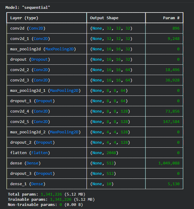
👁 cifar1 Output Step 5: Build the CNN Model Convolutional layers extract important spatial features from images. MaxPooling reduces the feature map size and computational load. Dropout helps prevent overfitting by randomly disabling neurons during training. Softmax layer produces probability scores for the 10 CIFAR-10 classes. Step 6: Compile the Model Optimizer : Adam provides fast and stable convergence. Loss Function: Categorical cross-entropy is used for multiclass output. Metrics : Accuracy helps track model performance during training. Output:
👁 cifar2 Output Step 7: Train the Model Epochs : 30 training cycles for learning patterns effectively. Batch Size: 64 samples per batch for efficient gradient updates. Validation Split: Helps monitor overfitting and generalization. History Object: Stores accuracy and loss values for later visualization. Step 8: Plot Training History Check for overfitting or underfitting Visual representation helps debug training issues Output:
Model Accuracy Graph:
The training accuracy increases steadily with each epoch, showing that the model is learning patterns from the data. Validation accuracy also improves but starts to level off after some epochs. The small gap between training and validation accuracy suggests the model generalizes reasonably well, with only mild overfitting toward the end. Model Loss Graph:
Training loss consistently decreases, meaning the model’s predictions are getting better on training data. Validation loss drops initially but then fluctuates slightly, indicating that learning has stabilized. This behavior shows the model has mostly converged, and further training may not give significant improvement. Step 10: Predict on Test Images Use model.predict to get class probabilities Display predicted and true labels Output:
We can see our model is working fine.
You can download full code from here .
