This article will give you clarity on what is dimensionality reduction, its need, and how it works. There is also python code for illustration and comparison between PCA, ICA, and t-SNE.

What is Dimensionality Reduction and why do we need it?

Dimensionality Reduction is simply reducing the number of features (columns) while retaining maximum information. Following are reasons for Dimensionality Reduction:

Dimensionality Reduction helps in data compression, and hence reduced storage space.
It reduces computation time.
It also helps remove redundant features, if any.
Removes Correlated Features.
Reducing the dimensions of data to 2D or 3D may allow us to plot and visualize it precisely. You can then observe patterns more clearly.
It is helpful in noise removal also and as a result of that, we can improve the performance of models.

How does Dimensionality Reduction works (using PCA)?

There are many methods for Dimensionality Reduction like PCA, ICA, t-SNE, etc., we shall see PCA (Principal Component Analysis).

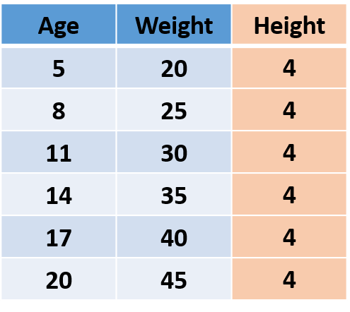
Let’s first understand what is information in data. Consider the following imaginary data, which has Age, Weight, and Height of people.

👁 Data PCA

Fig.1

The information lies in the variance!

As the ‘Height’ of all the people is the same i.e. the variance is 0 thus it’s not adding any information, so we can remove the ‘Height’ column without losing any information.

Now we know that information is variance, let’s understand the working of PCA. In PCA, we find new dimensions (features) that capture maximum variance (i.e. information). To understand this we shall use the previous example. After removing ‘Height’, we are left with ‘Age’ and ‘Weight’. These two features are caring all the information. In other words, we can say that we require 2 features (Age and Height) to hold the information, and if we can find a new feature that alone can hold all the information, we can replace origination 2 features with a new single feature, achieving dimensionality reduction!

👁 PCA graph

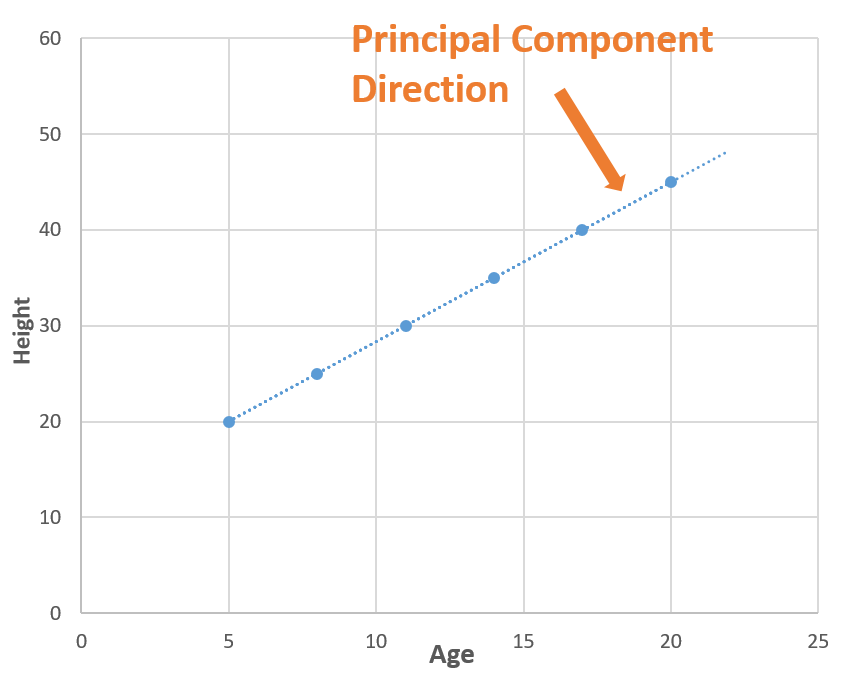
Now consider a line (blue dotted line) that is passing through all the points. The blue dotted line is capturing all the information so, we can replace ‘Age’ and ‘Weight’ (2 Dimensions) with the blue dotted line (1 Dimension) without losing any information, and in this way, we have done dimensionality reduction (2 dimensions to 1 dimension). The blue dotted line is called Principal Component.

You make be wondering how did we find the blue dotted line (Principal Component), so there is a lot of mathematics playing behind it. You can read this articlewhich explains this, but in simple words, we find the directions in which we can capture maximum variance using Eigenvalues and Eigenvectors.

PCA illustration in Python

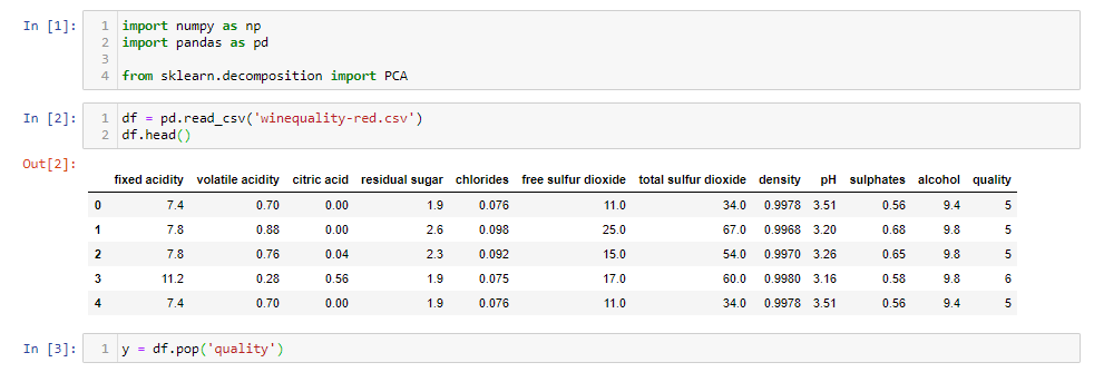
Let’s see how to use PCA with an example. I have used wine quality data which has 12 features like acidity, residual sugar, chlorides, etc., and the quality of the wine for 1600 samples. You can download the jupyter notebook from here and follow along.

First, let’s load the data.

import numpy as np
import pandas as pd
from sklearn.decomposition import PCA

df = pd.read_csv('winequality-red.csv')
df.head()
y = df.pop('quality')

👁 PCA import data

After loading the data, we removed the ‘Quality’ of the wine as it is the target feature. Now we will scale the data because if not PCA will not be able to find the optimal Principal Components. For eg. we have a feature in ‘meters’ and another in ‘kilometers’, the feature with unit ‘meter’ will have more variance than ‘kilometers’ (1 km = 1000 m), so PCA will give more importance to the feature with high variance. So, let’s do the scaling.

from sklearn.preprocessing import StandardScaler
scalar = StandardScaler()
df_scaled = pd.DataFrame(scalar.fit_transform(df), columns=df.columns)
df_scaled

import pandas as pd
df = pd.read_csv('winequality-red.csv')

y = df.pop('quality')


from sklearn.preprocessing import StandardScaler
scalar = StandardScaler()
df_scaled = pd.DataFrame(scalar.fit_transform(df), columns=df.columns)
print(df_scaled)

Now we are ready to apply for PCA.

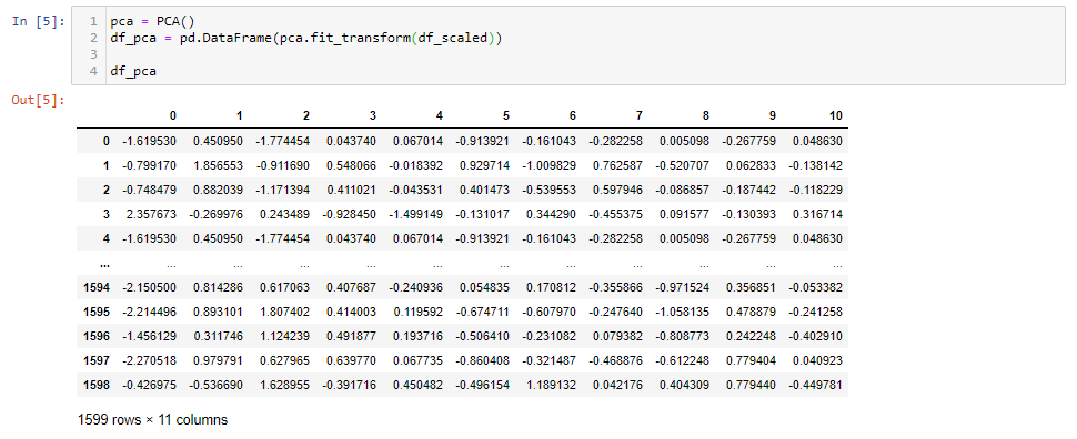
pca = PCA()
df_pca = pd.DataFrame(pca.fit_transform(df_scaled))
df_pca

👁 PCA

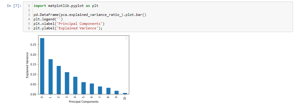
After applying PCA, we got 11 Principal Components. It’s interesting to see how much variance each principal component captures.

import matplotlib.pyplot as plt
pd.DataFrame(pca.explained_variance_ratio_).plot.bar()
plt.legend('')
plt.xlabel('Principal Components')
plt.ylabel('Explained Varience');

👁 Graph

The first 5 Principal Components are capturing around 80% of the variance so we can replace the 11 original features (acidity, residual sugar, chlorides, etc.) with the new 5 features having 80% of the information. So, we have reduced the 11 dimensions to only 5 dimensions while retaining most of the information.

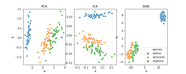
Difference between PCA, ICA, and t-SNE

PCA can also be used for clustering. I have used the iris dataset for this purpose. The following image will show you the clustering using PCA, ICA, and t-SNE.

👁 PCA, ICA, and t-SNE

As this article focuses on the basic ideas behind dimensionality reduction and working of PCA, we will not go into the details but those who are interested can go through this article.

In short, PCA does dimensionality reduction while capturing most of the variance. Now, you would be excited to apply PCA to your data but before that, I want to highlight some of the disadvantages of PCA: