Introduction
. Mindless about the different features present in the dataset, how we make the best out of the data is what affects the performance of the forecasting model on a large basis.
So how do we exhibit our data to leverage it for a specific application? ……. Feature Engineering
Feature Engineering
Feature engineering is one of the important tasks that need to be performed in designing any data science-related problem statement because exhibiting the data in a proper way can have an enormous influence on the evaluation of the model. In other words, this method involves experimenting with all combinations of features to highlight the key ones thereby isolating those that are irrelevant. It requires domain knowledge for selecting the most appropriate features that will bring out an accurate result.
Feature Selection
Feature selection or variable selection is a cardinal process in the feature engineering technique which is used to reduce the number of dependent variables. This is achieved by picking out only those that have a paramount effect on the target attribute. By employing this method, the exhaustive dataset can be reduced in size by pruning away the redundant features that reduce the model’s accuracy. Doing this will help curtail the computational expense of modeling and in some cases may also boost the accuracy of the implemented model.
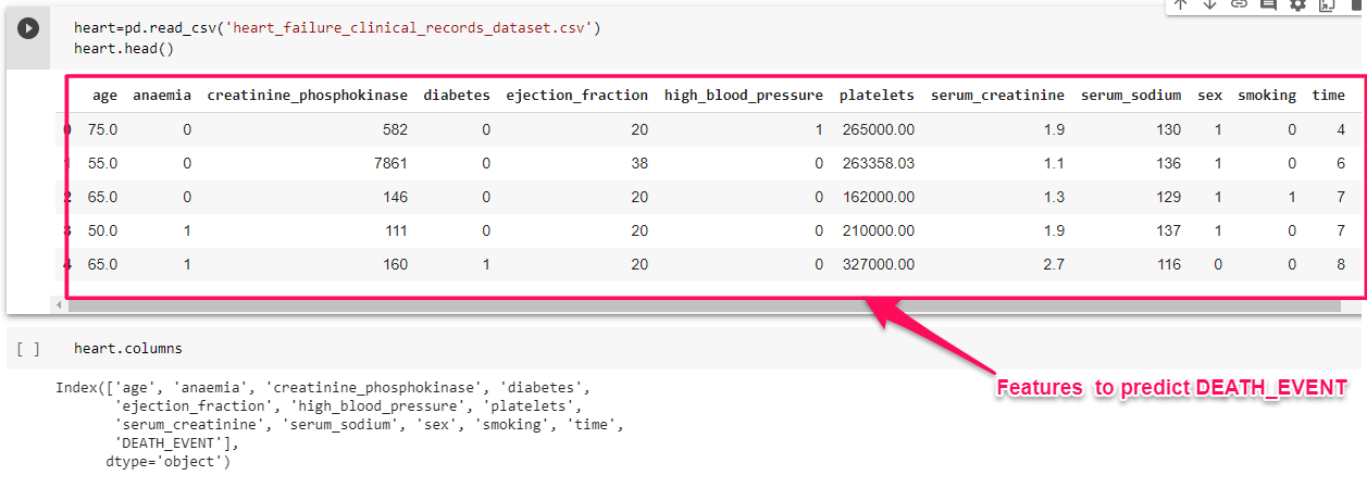
For example let us consider, Heart Failure Clinical dataset containing medical records of patients who had left ventricular systolic dysfunction and with a history of heart failure.
So here we have 12 features enlisted to carry out the forecasting process. Clearly using our expertise in this field we can tell that whether a person suffers from heart failure or not can be predicted using the Gender of the person. Nowadays a person irrespective of age and gender is suffering from CVD, so it may not be a key feature for prediction and hence can be isolated from training the model.
Increasing the features can make the model complex to learn and can also cause overfitting. In order to generalize the feature selection methods/models, we will look into a few feature selection techniques to reduce the dimensionality of the dataset. There are 3 basic approaches: Model-based approach(Extra-tree classifier), Iterative search (Forward stepwise selection), and Univariant statistics (Correlation and Chi-square test).
The feature selection methods we are going to discuss encompasses the following:
- Extra Tree Classifier
- Pearson correlation
- Forward selection
- Chi-square
- Logit (Logistic Regression model)
Extra Tree Classifier
This is a Model-based approach for selecting the features using the tree-based supervised models to make decisions on the importance of the features. The Extra Tree Classifier or the Extremely Random Tree Classifier is an ensemble algorithm that seeds multiple tree models constructed randomly from the training dataset and sorts out the features that have been most voted for. It fits each decision tree on the whole dataset rather than a bootstrap replica and picks out a split point at random to split the nodes.
The splitting of nodes occurring at every level of the constituent decision trees is based on the measure of randomness or entropy in the sub-nodes. The nodes are split on all variables available in the dataset and the split that results in the most homogenous sub-child is selected in the constituent tree models. This lowers the variance and makes the model less prone to overfitting.
X=heart.iloc[:,0:12]
Y=heart['DEATH_EVENT']
from sklearn.ensemble import ExtraTreesClassifier
model = ExtraTreesClassifier()
model.fit(X, Y)
print(model.feature_importances_)
feat_importances = pd.Series(model.feature_importances_, index=X.columns)
feat_importances.nlargest(13).plot.bar()
plt.show()
list1=feat_importances.keys().to_list()
Pearson Correlation
Pearson Correlation is used to construct a correlation matrix that measures the linear association between two features and gives a value between -1 and 1 indicating how related the two features are to one another. This measures the degree to which two features are interdependent by computing the association between each feature and the target variable, the one exerting high impact on the target can be picked out.
where x is the ith value of the variable x, xis the average value of sample attribute x, n is the number of records in the dataset and, x and y are the independent and target variables. A value of 1 indicates a positive correlation, -1 indicates a negative correlation and 0 indicates no correlation between the features.
#Correlation with the output variable
cor_target = abs(corr["DEATH_EVENT"])
#Selecting highly correlated features
relevant_features = cor_target[cor_target>0.2]
list4=relevant_features.keys().to_list()
list4
Chi-squared
A chi-square test is used in statistical models to check the independence of attributes. The model measures the degree of deviation between the expected and actual response. The lower the value of Chi-square, the less dependent the variables are to one another, and the higher the value more is their correlation. Initially, the attributes are assumed to be independent which forms the null hypothesis. The value of the expected outcome is computed using the following formula:
Chi-square is obtained from the expression that goes as follows:
Where, i is in the range (1,n), n is the number of dataset records, Oi is the actual outcome, and Eiis the expected outcome.
chi2_features = SelectKBest(chi2, k = 6)
X_kbest_features = chi2_features.fit_transform(X, Y)
mask=chi2_features.get_support()
new_feature=[]
for bool,feature in zip(mask,X.columns):
 if bool:
 new_feature.append(feature)
list3=new_feature
list3
Forward Selection
Forward selection is a wrapper model that evaluates the predictive power of the features jointly and returns a set of features that performs the best. It selects the predictors one by one and chooses that combination of features that makes the model perform the best based on the cumulative residual sum of squares. This process continues till there is no impact on the performance of the model with the incoming variable.
from sklearn.ensemble import RandomForestRegressor, RandomForestClassifier
from sklearn.metrics import roc_auc_score
from mlxtend.feature_selection import SequentialFeatureSelector
forward_feature_selector = SequentialFeatureSelector(RandomForestClassifier(n_jobs=-1),
 k_features=6,
 forward=True,
 verbose=2,
 scoring='roc_auc',
 cv=4)
fselector = forward_feature_selector.fit(X,Y)
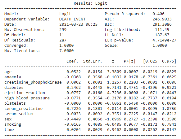
Logit Model
This is the Logistic regression-based model which selects the features based on the p-value score of the feature. The features with p-value less than 0.05 are considered to be the more relevant feature.
import statsmodels.api as sm
logit_model=sm.Logit(Y,X)
result=logit_model.fit()
print(result.summary2())
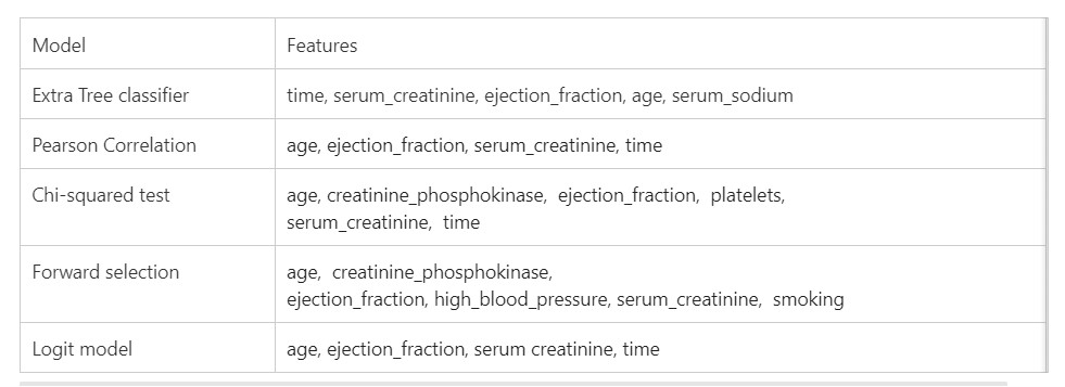
Now we have applied different feature selection models to our dataset, we will see the features selected by each module,
Now that the features have been selected, we are good to apply any supervised classification models to predict the outcome.
You can find the full code of this project
here.
Happy learning !!
You can reach out to me through LinkedIn
The media shown in this article on feature selection methods are not owned by Analytics Vidhya and is used at the Author’s discretion.

.png)
.png)
.png)