Simple understanding and implementation of KNN algorithm!

5 min read

Overview:

K Nearest Neighbor (KNN) is intuitive to understand and an easy to implement the algorithm. Beginners can master this algorithm even in the early phases of their Machine Learning studies.

This KNN article is to:

· Understand K Nearest Neighbor (KNN) algorithm representation and prediction.

· Understand how to choose K value and distance metric.

· Required data preparation methods and Pros and cons of the KNN algorithm.

· Pseudocode and Python implementation.

Introduction:

K Nearest Neighbor algorithm falls under the Supervised Learning category and is used for classification (most commonly) and regression. It is a versatile algorithm also used for imputing missing values and resampling datasets. As the name (K Nearest Neighbor) suggests it considers K Nearest Neighbors (Data points) to predict the class or continuous value for the new Datapoint.

The algorithm’s learning is:

1. Instance-based learning: Here we do not learn weights from training data to predict output (as in model-based algorithms) but use entire training instances to predict output for unseen data.

2. Lazy Learning: Model is not learned using training data prior and the learning process is postponed to a time when prediction is requested on the new instance.

3. Non -Parametric: In KNN, there is no predefined form of the mapping function.

How does KNN Work?

1. 
   

   Principle:

   
   

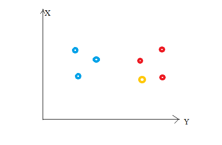
   Consider the following figure. Let us say we have plotted data points from our training set on a two-dimensional feature space. As shown, we have a total of 6 data points (3 red and 3 blue). Red data points belong to ‘class1’ and blue data points belong to ‘class2’. And yellow data point in a feature space represents the new point for which a class is to be predicted. Obviously, we say it belongs to ‘class1’ (red points)

   
   

   Why?

   
   

   Because its nearest neighbors belong to that class!

   
   

   👁 KNN algorithm image
   

   
   

   
   
   
   
   

   Yes, this is the principle behind K Nearest Neighbors. Here, nearest neighbors are those data points that have minimum distance in feature space from our new data point. And K is the number of such data points we consider in our implementation of the algorithm. Therefore, distance metric and K value are two important considerations while using the KNN algorithm. Euclidean distance is the most popular distance metric. You can also use Hamming distance, Manhattan distance, Minkowski distance as per your need. For predicting class/ continuous value for a new data point, it considers all the data points in the training dataset. Finds new data point’s ‘K’ Nearest Neighbors (Data points) from feature space and their class labels or continuous values.

   
   

   Then:

   
   

   For classification: A class label assigned to the majority of K Nearest Neighbors from the training dataset is considered as a predicted class for the new data point.

   
   

   For regression: Mean or median of continuous values assigned to K Nearest Neighbors from training dataset is a predicted continuous value for our new data point

   
   
   
2. 
   

   Model Representation

   
   
   

   Here, we do not learn weights and store them, instead, the entire training dataset is stored in the memory. Therefore, model representation for KNN is the entire training dataset.

   
   

K is a crucial parameter in the KNN algorithm. Some suggestions for choosing K Value are:

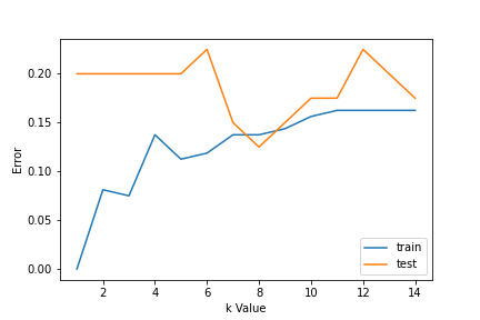
1. Using error curves: The figure below shows error curves for different values of K for training and test data.

At low K values, there is overfitting of data/high variance. Therefore test error is high and train error is low. At K=1 in train data, the error is always zero, because the nearest neighbor to that point is that point itself. Therefore though training error is low test error is high at lower K values. This is called overfitting. As we increase the value for K, the test error is reduced.

But after a certain K value, bias/ underfitting is introduced and test error goes high. So we can say initially test data error is high(due to variance) then it goes low and stabilizes and with further increase in K value, it again increases(due to bias). The K value when test error stabilizes and is low is considered as optimal value for K. From the above error curve we can choose K=8 for our KNN algorithm implementation.

2. Also, domain knowledge is very useful in choosing the K value.

3. K value should be odd while considering binary(two-class) classification.

Required Data Preparation:

1. Data Scaling: To locate the data point in multidimensional feature space, it would be helpful if all features are on the same scale. Hence normalization or standardization of data will help.

2. Dimensionality Reduction: KNN may not work well if there are too many features. Hence dimensionality reduction techniques like feature selection, principal component analysis can be implemented.

3. Missing value treatment: If out of M features one feature data is missing for a particular example in the training set then we cannot locate or calculate distance from that point. Therefore deleting that row or imputation is required.

Python implementation:

Implementation of the K Nearest Neighbor algorithm using Python’s scikit-learn library:

Step 1: Get and prepare data

import pandas as pd
import numpy as np
import matplotlib.pyplot as plt
from sklearn.datasets import make_classification
from sklearn.model_selection import train_test_split
from sklearn.preprocessing import StandardScaler
from sklearn.neighbors import KNeighborsClassifier 
from sklearn import metrics

After loading important libraries, we create our data using sklearn.datasets with 200 samples, 8 features, and 2 classes. Then data is split into the train(80%) and test(20%) data and scaled using StandardScaler.

Python Code:

import pandas as pd
import numpy as np
import matplotlib.pyplot as plt
from sklearn.datasets import make_classification
from sklearn.model_selection import train_test_split
from sklearn.preprocessing import StandardScaler
from sklearn.neighbors import KNeighborsClassifier 
from sklearn import metrics

X,Y=make_classification(n_samples= 200,n_features=8,n_informative=8,n_redundant=0,n_repeated=0,n_classes=2,random_state=14)
X_train, X_test, y_train, y_test= train_test_split(X, Y, test_size= 0.2,random_state=32)
sc= StandardScaler()
sc.fit(X_train)
X_train= sc.transform(X_train)
sc.fit(X_test)
X_test= sc.transform(X_test)
print(X.shape)

(200, 8)

Step 2: Find the value for K

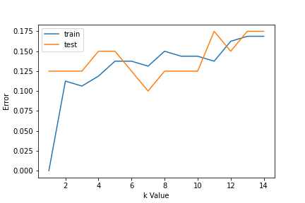
For choosing the K value, we use error curves and K value with optimal variance, and bias error is chosen as K value for prediction purposes. With the error curve plotted below, we choose K=7 for the prediction 

error1= []
error2= []
for k in range(1,15):
 knn= KNeighborsClassifier(n_neighbors=k)
 knn.fit(X_train,y_train)
 y_pred1= knn.predict(X_train)
 error1.append(np.mean(y_train!= y_pred1))
 y_pred2= knn.predict(X_test)
 error2.append(np.mean(y_test!= y_pred2))
# plt.figure(figsize(10,5))
plt.plot(range(1,15),error1,label="train")
plt.plot(range(1,15),error2,label="test")
plt.xlabel('k Value')
plt.ylabel('Error')
plt.legend()

Step 3: Predict:

In step 2, we have chosen the K value to be 7. Now we substitute that value and get the accuracy score = 0.9 for the test data.

knn= KNeighborsClassifier(n_neighbors=7)
knn.fit(X_train,y_train)
y_pred= knn.predict(X_test)
metrics.accuracy_score(y_test,y_pred)

0.9

Pseudocode for K Nearest Neighbor (classification):

Login to continue reading and enjoy expert-curated content.

Free Courses

Become an Author

Share insights, grow your voice, and inspire the data community.

• Reach a Global Audience
• Share Your Expertise with the World
• Build Your Brand & Audience

• Join a Thriving AI Community
• Level Up Your AI Game
• Expand Your Influence in Genrative AI

👁 imag