Outlier detection is one of the widely used methods in any data science project, as its presence can lead to the development of a bad machine learning model. Let’s take a quick scenario of the linear regression problem statement, where suppose you have to predict the person’s weight from the height. In general, one with more height will also have more weight (linear positive trend), but what if rarely we have 3-4 people who have much less weight, but comparatively more height than that data will be treated as bad data or the outliers. Which, in the end, would not be a good fit for our regression model.

There are various ways through which we can deal with the outliers, though, in this article, we will have our complete focus on the Z-Score method. Here we will talk about the limitations of this method, When to use and prefer other methods, and of course, the complete implementation using Python.

👁 outliers

Source: Analytics Vidhya

Limitations of Z-Score

Though Z-Score is a highly efficient way of detecting and removing outliers, we cannot use it with every data type. When we said that, we mean that it only works with the data which is completely or close to normally distributed, which in turn stimulates that this method is not for skewed data, either left skew or right skew. For the other data, we have something known as Inter quartile range (IQR) method, which we will cover in the next article in depth.

Enough of the theory. Let’s now jump to practically implement this method and see how we can detect and remove the bad data from the dataset to improve the model accuracy.

import numpy as np
import pandas as pd
import matplotlib.pyplot as plt
import seaborn as sns

We prepare our stuff by importing all the essential libraries from Python’s supported package. Here we have imported four main libraries that we will use during the execution part:

Numpy: For performing mathematical calculations by simplifying the same from its predefined functions
Pandas: Pandas is the data manipulation library that helps play with DataFrames.
Matplotlib: This is one of the most common libraries used for visualization closest to the python backend.
Seaborn: Another visualization library with better representation, look, and feel but built on top of matplotlib.

df_org = pd.read_csv('placement.csv')
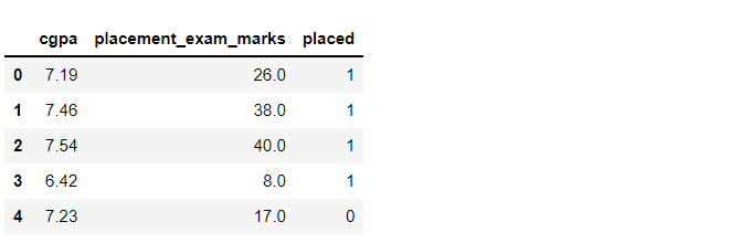
df_org.head()

Output:

👁 Image

Inference: We are using the simple placement dataset for this article where we will take GPA and placement exam marks as two columns and select one of the columns which will show the normal distribution, then will proceed further to remove outliers from that feature. Use the head function to show the top 5 rows.

df_org.shape

Output:

(1000, 3)

Inference: As the shape function stimulates, we have 1000 rows of data with 3 columns -> (1000,3).

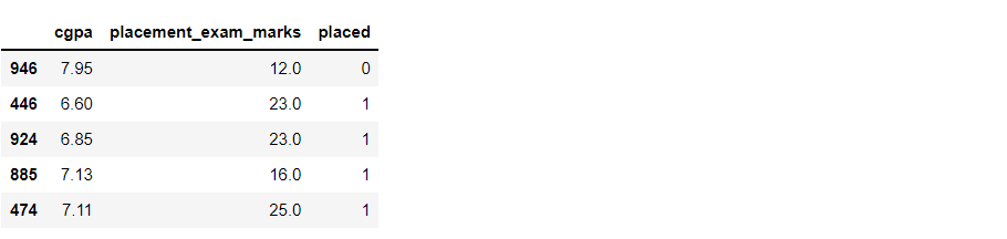
df_org.sample(5)

Output:

👁 outliers

Inference: Like head function returns the top 5 rows (by default). Similarly, the sample function returns the random sample of ‘n’ rows depending on what value we are giving in the parameter.

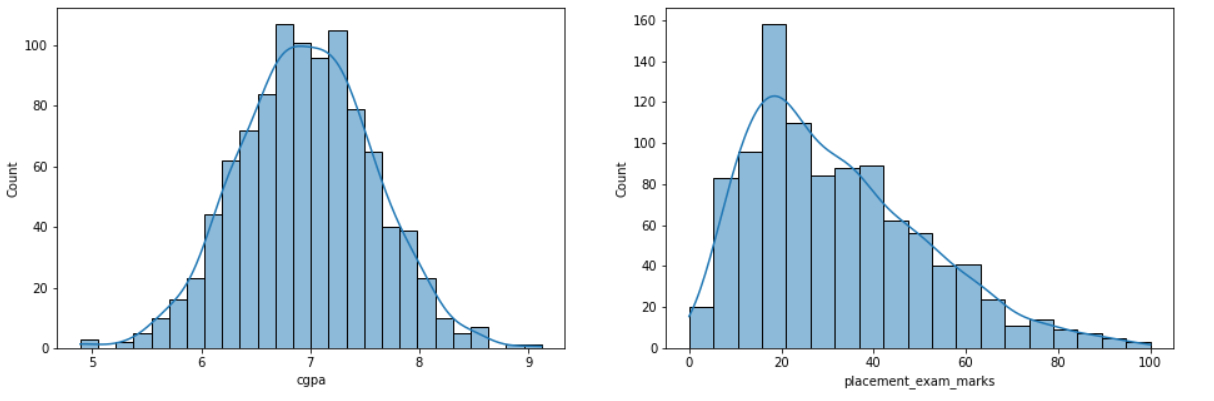
plt.figure(figsize=(16,5))
plt.subplot(1,2,1)
sns.histplot(df_org['cgpa'], kde=True)

plt.subplot(1,2,2)
sns.histplot(df_org['placement_exam_marks'], kde=True)

plt.show()

Output:

👁 outliers

Inference: We chose hist-plot with kernel density as a True graph for both CGPA and placement_exam_marks column so that we can clearly understand that among them, which one has the normal distribution?

From the graph, we can see that CGPA is almost the right fit for the normal distribution, or we can say it is forming the correct bell curve. Meanwhile, the other one is slightly skewed towards the right. Hence, we are gonna take CGPA for our further analysis.

df_org['placement_exam_marks'].skew()

Output:

0.8356419499466834

df_org['cgpa'].skew()

Output:

-0.014529938929314918

Inference: We were lucky enough to spot the difference between a normal distribution and skewed distribution from the above graph, but sometimes, the graph might not give a clear understanding that we have the skew function from pandas which will give a higher positive value if the distribution seems to be skewed (placement_exam_marks) otherwise it will return the quite lower value even in negative if it is not skewed at all (CGPA).

print("Mean value of cgpa",df_org['cgpa'].mean())
print("Standard deviation of cgpa",df_org['cgpa'].std())
print("Minimum value of cgpa",df_org['cgpa'].min())
print("Maximum value of cgpa",df_org['cgpa'].max())

Output:

Mean value of cgpa 6.96124000000001
Standard deviation of cgpa 0.6158978751323894
Minimum value of cgpa 4.89
Maximum value of cgpa 9.12

Inference: Here are some different statistical measures for CGPA, which are printed out to compare the original values (from original data) to when the data will be free of any outlier. The analysis will also be evident.

Approach for Outliers

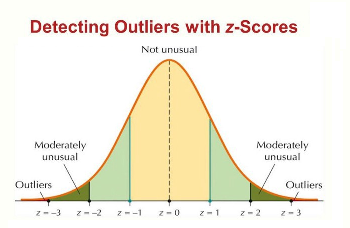
From here onwards, our main task starts, but before implementing the same, let’s first discuss the game plan and how we will approach dealing with bad data using Z-Score:

The very first step will be setting the upper and lower limit. This range stimulates that every data point will be regarded as an outlier out of this range. Let’s see the formulae for both upper and lower limits.
- Upper: Mean + 3 * standard deviation.
- Lower: MEan – 3 * standard deviation.

print("Upper limit",df_org['cgpa'].mean() + 3*df_org['cgpa'].std())
print("Lower limit",df_org['cgpa'].mean() - 3*df_org['cgpa'].std())

Output:

Upper limit 8.808933625397177
Lower limit 5.113546374602842

Inference: In the output, we see that the highest value is 8.80 while the lowest value is 5.11. Hence any value out of this range is the bad data point

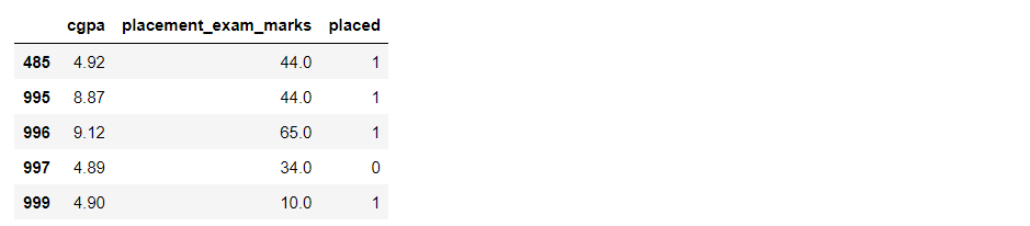
The second step is to detect how many outliers are there in the dataset based on the upper and lower limit that we set up just

df_org[(df_org['cgpa'] > 8.80) | (df_org['cgpa'] < 5.11)]

Output:

👁 dataset

Inference: Now, we are performing the filtering using pandas where we are passing in two conditions keeping in mind that if either condition is True, then our objective will be attained. In the output, we can see that it returned 5 rows, i.e., 5 outliers in the dataset.

Now, we are gonna start with the third and the last step, where we will finally remove the detected outliers in step 2 using two techniques; we can either go for Trimming or Capping, and we will discuss both techniques more closely separately.

Trimming for Outliers

The first technique for dealing with outliers is trimming, and this is regardless of what kind of data distribution you are working with, trimming is an applicable and proven technique for most data types. We pluck out all the outliers using the filter condition in this technique.

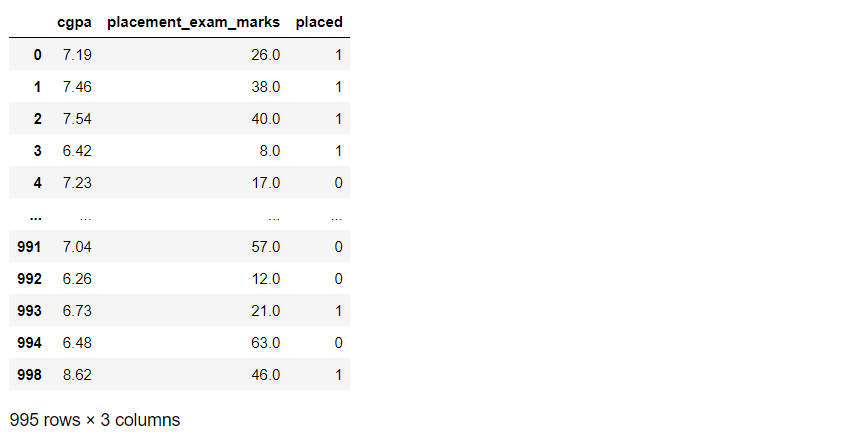
new_df_org = df_org[(df_org['cgpa'] 5.11)]
new_df_org

Output:

👁 outliers

Inference: So, as we can see, we applied that condition where all the data should be in the range of our upper and lower limit. As a result, instead of 1000 rows, it returned 995 rows which indicate that we have successfully removed 5 outliers.

Capping

Capping is another technique for dealing with bad data points; it is useful when we have many outliers, and removing a good amount of data from the dataset is not good. In that case, capping comes into the picture as it won’t remove them. Instead, it brings back those data points within the range we specified according to our Z-Score value.

upper_limit = df_org['cgpa'].mean() + 3*df_org['cgpa'].std()
lower_limit = df_org['cgpa'].mean() - 3*df_org['cgpa'].std()

df_org['cgpa'] = np.where(
 df_org['cgpa']>upper_limit,
 upper_limit,
 np.where(
 df_org['cgpa']<lower_limit,
 lower_limit,
 df_org['cgpa']
 )
)

Inference: The first thing is setting the upper and lower bound. Then comes the part of np. Where the function that will help to implement the logic behind capping, the basic syntax is as, np.where(condition, True, False) i.e., if the condition is true, then that data point will be getting the upper limit value (within range) if not, it will go to check the lower limit, and if that’s true, then it will give that data point lower limit value (within range).

df_org.shape

Output:

(1000, 3)

Inference: As we did capping, no data was lost, and we still have 1000 rows.

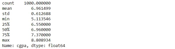
df_org['cgpa'].describe()

Output:

👁 outliers

Inference: Now, if we compare the minimum and maximum values before outlier removal and after, we can see that the minimum value is increased and the maximum value is decreased.

Conclusion

In this article, we discussed one of the efficient ways of dealing with and removing the bad data for our further analysis, i.e., removing outliers, also known as Anamoly detection. Here we saw how statistical measures such as Z-Score can help deal with such problems.

Firstly we started by importing libraries, reading the dataset, and having a brief look over it. Before that, we also discussed the limitations of Z-Score and when we should prefer it.
Then we analyze the data distribution of the columns to choose the normally distributed column as Z-Score only applies to that type. As a result, GPA seems to be fit for further analysis.
At last, we discussed two methods via which we can do the Anamoly detection: Trimming (removing outliers) and Capping (imputing outliers).

Here’s the repo link to this article. I hope you liked my article on Dealing with outliers using the Z-Score method. If you have any opinions or questions, comment below.

Connect with me on LinkedIn for further discussion on Python for Data Science or otherwise.

The media shown in this article is not owned by Analytics Vidhya and is used at the Author’s discretion.

👁 Aman Preet

Aman Preet

Beginner Data Exploration Machine Learning Python Python Statistics