Beginner’s Guide to Missing Value Ratio and its Implementation

Introduction

Feature Selection plays a key role in reducing the dimensions of any dataset. There are various benefits of dimensionality reduction including reduced computational/training time of a dataset, lesser dimensions lead to better visualization, etc. And Missing Value Ratio is one of the basic feature selection techniques. In this article, we are going to cover this technique and later one will see its implementation in Python as well.

Note: If you are more interested in learning concepts in an Audio-Visual format, We have this entire article explained in the video below. If not, you may continue reading.

What is the Missing Value Ratio and how do we calculate it?

Let’s say we have a dataset where we want to predict the count of bikes that have been rented-

👁 Missing Value Ratio data

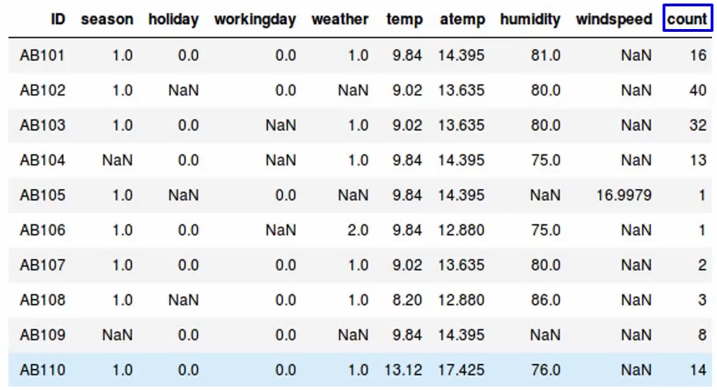
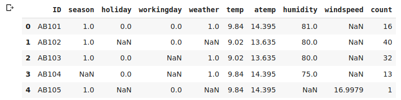
We have variables like the season, holiday, working day, weather, temperature, etc And our aim is to predict “the count” variable using all these independent variables. So what’s the first step you’ll take. We first explore the data and we find that there are a lot of missing values in our dataset-

👁 Missing Value Ratio nan values

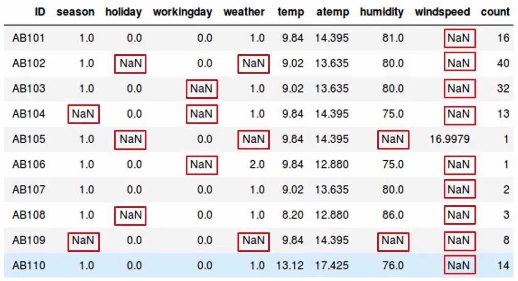
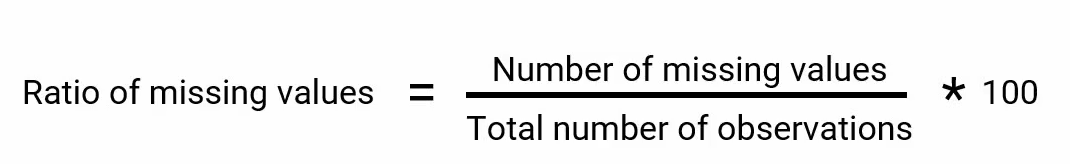
So we then decide to calculate the missing values. In each of these variables, we can calculate the ratio of missing values using a simple formula. The formula is- the number of missing values in each column divided by the total number of observation, and to calculate the percentage we’ll of course multiply this figure by a hundred-

👁 Missing Value Ratio formula

we can calculate this ratio for all the variables in our data-

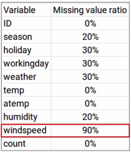
👁 Missing Value Ratio column wise

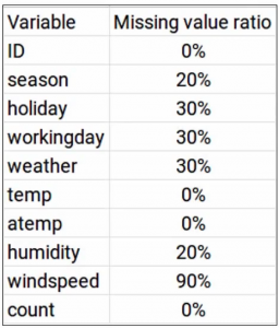
Once we have the missing value ratio on the variables, what’s the next step? Now we can decide a threshold, let’s say 70% and you can use this threshold and drop all the variables which have a missing value ratio more than this threshold. So when we look at a problem again-

👁 Missing Value Ratio windspeed

“the windspeed” variable has a missing value ratio of 90%, which is way more than a threshold of 70%. Hence, we can go ahead and drop this variable. Generally, we can draw variables having a missing value ratio of more than 60 or 70%.

Keep in mind that there’s no hard and fast rule to decide this threshold. And it can vary from problem to problem.

Once you drop the variables, which are missing values more than the threshold, how do you think we should deal with the remaining variables, which still have missing values in them? Should we just go ahead and remove all of them? Well, not quite in these scenarios, we should first try to find out the reason for the missing values.

It might be due to non-response or people refusing to share that particular information. It could be due to an error while collecting the data, or it could be due to the error in reading the data. There could be any number of reasons why you have missing values in the dataset. It’s important to find that out. Once we know the reason we will try to impute those missing values, we can use statistical measures like mean, median and mode, or we can even train a model to predict the missing values as well.

Implementing Missing Value Ratio

So this in a nutshell was how we can make use of missing values to reduce the dimensions in our dataset. It’s time to put learning into practice. Let’s power up a Jupiter notebook and implement it-

The very first step, import pandas-

#importing the libraries

import pandas as pd

Then read the dataset and use the data.head() function to look at the first five rows of our data-

#reading the file
data = pd.read_csv('missing_value_ratio-200306-192816.csv')

#first 5 rows of the data
data.head()

We saw earlier that we have a bunch of variables and the target variable count.

Let’s go ahead and print the shape of the data. Here we go-

#shape of the data

data.shape

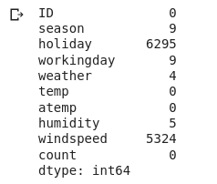
We have 12,980 observations and 10 variables or columns. Next, we will check the number of missing values in each column-

#number of missing values in each variable

data.isnull().sum()

Here you can see that holiday and windspeed seem to have a very high number of missing observations. The variables season, working day, weather, and humidity, also have missing values, as you can see, but they’re pretty negligible compared to holiday and windspeed.

To make this a little easier for ourselves, we’ll convert this into a percentage number-

# percentage of missing values in each variable

data.isnull().sum()/len(data)*100

As we saw above holiday and wind speed have over 40% missing values. It’s quite a lot. Generally, if a variable has around 40 to 50% missing values, you would want to impute them using either of the methods that we have discussed earlier.

But as the aim of this video is to make you understand how we can apply the missing value filter to reduce the dimensionality of the data set. We’ll set a threshold of 40% and then drop the variables having missing values more than this threshold.

Makes sense!

Let’s move on and save these percentages into a variable which we’ll call a and the column names in a variable called variables.

# saving missing values in a variable
a = data.isnull().sum()/len(data)*100

# saving column names in a variable
variables = data.columns

Now comes the interesting part. We will use a for-loop here to apply the threshold value on our data dataset. As I said earlier, I’m setting the threshold as 40%, but this can vary depending on the kind of problem you’re working with-

# new variable to store variables having missing values less than a threshold

variable = [ ]

for i in range(data.columns.shape[0]):
 if a[i]<=40: #setting the threshold as 40%
 variable.append(variables[i])

Let’s print out this new variable-

variable

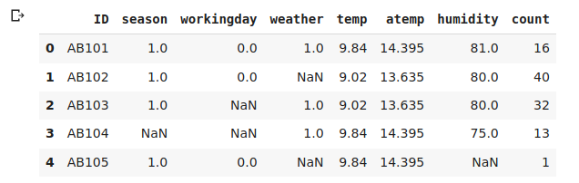
As we expected the holiday and windspeed variables have been dropped since they went above our threshold value of 40%. We’ll put the remaining variables into a new data frame and we’ll call it new_data. And let’s just check out the first five observations on this-

# creating a new dataframe using the above variables

new_data = data[variable]
new_data.head()

Yup. All according to plan, let’s verify the percentage of missing values in each variable of the new_data.

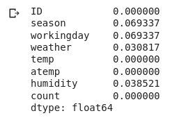
# percentage of missing values in each variable of new data

new_data.isnull().sum()/len(new_data)*100

Perfect! Finally, compare the shape of our new_data with the original dataset-

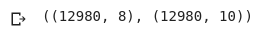
# shape of new and original data

new_data.shape, data.shape

👁 shape of new and original data

As you might’ve guessed already, the number of observations is the same, but there are two fewer variables in the new dataset. And this is how we can perform the missing value ratio in Python.

End Notes

In this article, I covered one of the most common feature selection techniques Missing Value Ratio. We saw the formula to calculate it and also its implementation in Python.

If you are looking to kick start your Data Science Journey and want every topic under one roof, your search stops here. Check out Analytics Vidhya’s Certified AI & ML BlackBelt Plus Program

If you have any queries, let me know in the comment section!

Login to continue reading and enjoy expert-curated content.

Free Courses