5 Hyperparameter Optimization Techniques You Must Know for Data Science Hackathons 

Introduction

1. 1. GridSearchCV
   2. RandomizedSearchCV
   3. Bayesian Optimization
   4. HyperOpt
   5. Optuna

For the python code, I used the Iris dataset which is available within the Scikit-learn package.

It is a very small dataset (150 rows only) with a multiclass classification problem. let us load the dataset and divide it into the independent feature and target feature. 

#importing packages
import pandas as pd
import numpy as np
from sklearn.datasets import load_iris

#Loading iris dataset from sklearn
iris = load_iris()

#Creating independent features
X = iris.data

#Creating traget features
y = iris.target

As we are mostly focussing on hyperparameter tuning, I have not performed the EDA(exploratory data analysis) or feature engineering part and directly jumped into the model-building. I used the XGBoostClssifier algorithm for the model-building to classify the target variables.

#Importing XGBoost
from xgboost import XGBClassifier

#Defining XGB classification model
clf = XGBClassifier()

1. GridSearchCV

GridSearchCV is a function that comes in Scikit-learn’s(or SKlearn) model_selection package.To use the GridSearchCV function, first, we define a dictionary in which we mention a particular hyperparameter along with the values it can take. Then, we pass predefined values for hyperparameters to the GridSearchCV function. We can set for coss validation for testing within this function.

#Importing packages from sklearn

from sklearn import preprocessing

from sklearn import model_selection

from sklearn import metrics

#defining a set of values as a dictionary for hyperparameters

param_grid = {

 "n_estimators":[100,200,300,400],

 "max_depth":[1,3,5,7],

 "reg_lambda":[.01,.1,.5] 

}

#declaring GridSearchCV model

model = model_selection.GridSearchCV(

 estimator = clf,

 param_grid = param_grid,

 scoring = 'accuracy',

 verbose = 10,

 n_jobs = 1,

 cv = 5 

)

#fitting values to the gridsearchcv model

model.fit(X,y)

#printing the best possible values to enhance accuracy

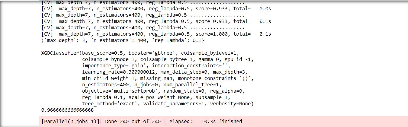
print(model.best_params_)

print()

print(model.best_estimator_)

#printing the best score

print(model.best_score_)

It seems that our hyperparameter optimization worked well and our model is working with 96.67% accuracy.

However, as GridSearchCV explores every possible combination of hyperparameters for the provided dataset, it can be time-consuming.

The above didn’t take long as it was a very small dataset. It took 10.3 seconds to try all 240 combinations.

If we have large datasets, then GridSearchCV should be avoided.

2. RandomizedSearchCV

RandomizedSearchCV is another function that comes within Scikit-learn’s model_selection package for Hyperparameter Tuning. To use the RandomizedSearchCV function, we again define a dictionary in which we mention a particular hyperparameter along with the values it can take(same as GridSearchCV). Then, we pass predefined values for hyperparameters to the GridSearchCV function.

However, the main difference between GridSearchCV and RandomizedSearchCV is that in RandomizedSearchCV we can set a fixed number of iterations. The RandomizedSearchCV function will randomly choose parameters from the provided set of parameters and generate the best possible combination of hyperparameters of provided number of trials.

#defining a set of values as a dictionary for hyperparameters

param_grid = {

 "n_estimators":[100,200,300,400],

 "max_depth":[1,3,5,7],

 "reg_lambda":[.01,.1,.5] 

}

#declaring RandomizedSearchCV model

model = model_selection.RandomizedSearchCV(

 estimator = clf,

 param_distributions = param_grid,

 scoring = 'accuracy',

 verbose = 10,

 n_jobs = 1,

 cv = 5,

 n_iter=10

)

#fitting values to the RandomizedSearchCV model

model.fit(X,y)

#printing the best possible values to enhance accuracy

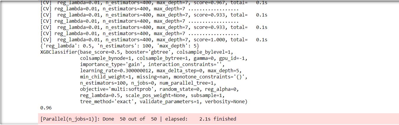
print(model.best_params_)

print(model.best_estimator_)

#printing the best score

print(model.best_score_)

In the above code, I have used n_iter=10(10 trials). RandomizedSearchCV picked 10 combinations among the provided hyperparameter list and produce the best combination of hyperparameters to optimize the model accuracy.

For the above code, RandomizedSearchCV resulted in an accuracy of 0.96 and it took 2.1 seconds to finish(for GridSearCV it was 10.3 seconds). We cannot see much difference in time as it is a very small dataset. However, for large datasets, the time difference is noticeable.

3. Bayesian Optimization

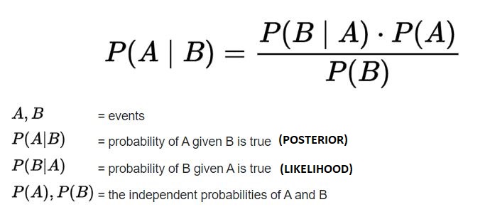
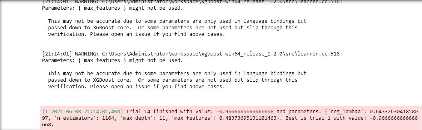
Bayesian optimization, as the name suggests works on Bayes Principle. Bayes’s principle basically says that posterior probability distribution is directly proportional to its priors (prior probability distribution) and the likelihood function.

Bayesian optimization is a global optimization method for noisy black-box functions. This technique is applied to hyperparameter optimization for ML models. Bayesian optimization builds a probabilistic model of the function mapping from hyperparameter values to the objective evaluated on a validation set. Without going into the theory in detail, let’s have a look at the python code for the Bayesian optimization method.

#importing packages 

from functools import partial

from skopt import space

from skopt import gp_minimize

#defining a method that will perfrom a 5 split cross validation over

#dataset and and will produce the optimum value of the accuracy

def optimize(params, param_names, x,y):

 params = dict(zip(param_names,params))

 model = XGBClassifier(**params)

 kf = model_selection.StratifiedKFold(n_splits=5)

 accuracies = []

 for idx in kf.split(X=x,y=y):

 train_idx,test_idx = idx[0],idx[1]

 xtrain = x[train_idx]

 ytrain = y[train_idx]

 xtest = x[test_idx]

 ytest = y[test_idx]

 model.fit(xtrain,ytrain)

 preds = model.predict(xtest)

 fold_acc = metrics.accuracy_score(ytest,preds)

 accuracies.append(fold_acc)

 return -1.0 * np.mean(accuracies)

#defining a set of values as space for hyperparameters

param_space = [

 space.Integer(3,15, name = "max_depth"),

 space.Integer(100,600, name = "n_estimators"),

 space.Real(0.01,1,prior='uniform', name="reg_lambda"),

 space.Real(0.01,1,prior='uniform', name="max_features")

]

#DEfining the parameter names

param_names = [

 "max_depth",

 "n_estimators",

 "reg_lambda",

 "max_features"

]

#defiing optimization_fuction as partial and calling optimize within it

optimization_fuction = partial(optimize, param_names = param_names,x = X, y = y) 

#Getting the optimum values for hyperparameters

result = gp_minimize(

 optimization_fuction,

 dimensions=param_space,

 n_calls = 15,

 n_random_starts= 10,

 verbose= 10

)

#Printing the best hyperparemeter set

print(dict(zip(param_names,result.x)))

Here I created one function named optimize. This function takes hyperparameter tuning parameters, independent dataset, and target feature as input parameters. It returns the optimum value according to the specified performance measures(for the above function, it is accuracy).

The hyperparameter values are provided within the space module of the skopt package.

Then, there is another function optimization_fuction (as partial) and we call optimize from within optimization_fuction.

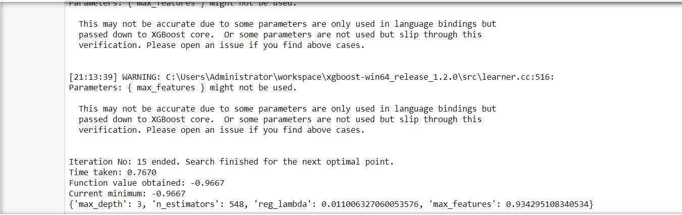
Finally, we optimize the parameter values by calling skopt.gp_minimize

The above code performed the optimization in 0.77 seconds and with an accuracy of 0.97%.

So far, this optimization technique showed better results than the earlier two models.

Here I would like to mention that I used StratifiedKFold for cross-validation in the above code as it was a classification problem. In the case of a regression problem, it would not work. In that case, we should use only KFold.

4. HyperOpt

HyperOpt is an open-source python library that is used for hyperparameter optimization for ML models. Like the other above-mentioned optimization methods, it searches through hyperparameter space.   following is the python code for HyperOpt implementation.  You can have a look at the documentation of this package to get a detailed idea about the parameters.

#importing packages 

from hyperopt import hp,fmin, tpe, Trials

from hyperopt.pyll.base import scope

from functools import partial

from skopt import space

from skopt import gp_minimize

#defining a method that will perfrom a 5 split cross validation over

#dataset and and will produce the optimum value of the accuracy

def optimize(params, x,y):

 clf = XGBClassifier(**params)

 kf = model_selection.StratifiedKFold(n_splits=5)

 accuracies = []

 for idx in kf.split(X=x,y=y):

 train_idx,test_idx = idx[0],idx[1]

 xtrain = x[train_idx]

 ytrain = y[train_idx]

 xtest = x[test_idx]

 ytest = y[test_idx]

 clf.fit(xtrain,ytrain)

 preds = clf.predict(xtest)

 fold_acc = metrics.accuracy_score(ytest,preds)

 accuracies.append(fold_acc)

 return -1.0 * np.mean(accuracies)

#defining a set of values as hp for hyperparameters

param_space = {

 "max_depth" : scope.int(hp.quniform("max_depth",3,20, 1)) ,

 "min_child_weight" : scope.int(hp.quniform("min_child_weight",1,8, 1)),

 "n_estimators": scope.int(hp.quniform("n_estimators",100,1500,1)),

 'learning_rate': hp.uniform("learning_rate",0.01,1),

 'reg_lambda': hp.uniform("reg_lambda",0.01,1),

 'gamma': hp.uniform("gamma",0.01,1),

 'subsample': hp.uniform("subsample",0.01,1)

 }

#defiing optimization_fuction as partial and calling optimize within it

optimization_fuction = partial(optimize,x = X, y = y) 

trials = Trials()

#Getting the optimum values for hyperparameters

result = fmin(

 fn = optimization_fuction,

 space = param_space,

 algo = tpe.suggest,

 max_evals = 15,

 trials = trials

)

#Printing the best hyperparemeter set

print(result)

The code for HyperOpt is similar to the Bayesian Optimization technique. The construction of optimize() function is almost similar. Although, here we don’t have to send the param_name in the parameter of the function. Also, the way we define param_space is different.

The above code took 0.12 seconds to execute and returned 0.96% accuracy. This also seems to be a good option for our code.

5.Optuna

Optuna is another open-source python library that is used for hyperparameter optimization for ML models. following is the python code for HyperOpt implementation.

#importing packages

import optuna

from functools import partial

#defining a method that will perfrom a 5 split cross validation over

#dataset and and will produce the optimum value of the accuracy

def optimize(trial, x,y):

 #parameter set is declare within function

 reg_lambda = trial.suggest_uniform('reg_lambda',0.01,1)

 n_estimators = trial.suggest_int('n_estimators',100,1500)

 max_depth = trial.suggest_int('max_depth',3,15)

 max_features = trial.suggest_uniform('max_features',0.01,1)

 clf = XGBClassifier(

 n_estimators= n_estimators,

 reg_lambda=reg_lambda,

 max_depth=max_depth,

 max_features= max_features)

 kf = model_selection.StratifiedKFold(n_splits=5)

 accuracies = []

 for idx in kf.split(X=x,y=y):

 train_idx,test_idx = idx[0],idx[1]

 xtrain = x[train_idx]

 ytrain = y[train_idx]

 xtest = x[test_idx]

 ytest = y[test_idx]

 clf.fit(xtrain,ytrain)

 preds = clf.predict(xtest)

 fold_acc = metrics.accuracy_score(ytest,preds)

 accuracies.append(fold_acc)

 return -1.0 * np.mean(accuracies)

#defiing optimization_fuction as partial and calling optimize within it

optimization_fuction = partial(optimize,x = X, y = y) 

study = optuna.create_study(direction='minimize')

#Printing the best hyperparemeter set

study.optimize(optimization_fuction, n_trials=15)

The coding for Optuna is a little bit different than Hyperopt. Here, we don’t have to declare any parameter set separately. We provide the set of hyperparameter values within the optimize function itself. The rest of the code is similar to the code for Hyperopt.

The above code took 0.11 seconds to execute and produced 0.97% accuracy.

The execution time for the above-mentioned optimization techniques may vary depending on the provided dataset size. You may choose any technique you like. However, for the complex algorithms(ex: boosting ones), I have observed that the former three optimization techniques(Bayesian Optimization, Hyperopt, Optuna)  perform better.

The media shown in this article on Hyperparameter Optimization Techniques are not owned by Analytics Vidhya and are used at the Author’s discretion.

Login to continue reading and enjoy expert-curated content.

Free Courses