Building a Logistic Regression model from scratch

Do you understand how does logistic regression work? If your answer is yes, I have a challenge for you to solve. Here is an extremely simple logistic problem.

X = { 1,2,3,4,5,6,7,8,9,10}

Y = {0,0,0,0,1,0,1,0,1,1}

Here is the catch : YOU CANNOT USE ANY PREDEFINED LOGISTIC FUNCTION!

Why am I asking you to build a Logistic Regression from scratch?

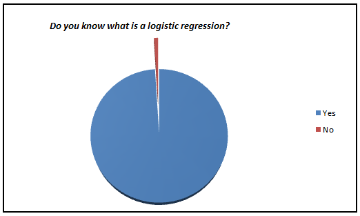
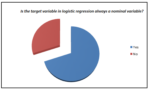
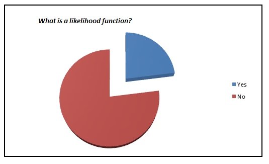
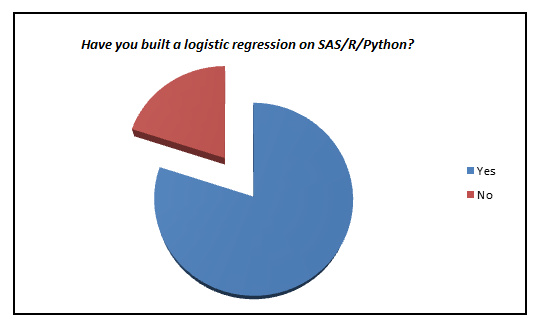
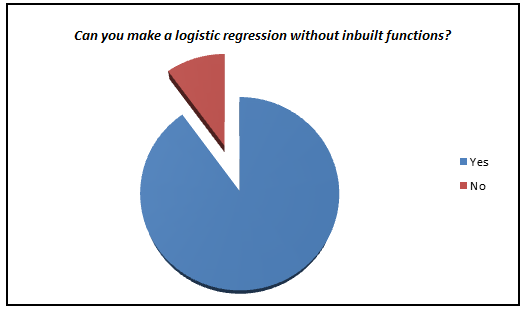
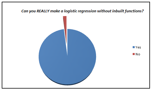
Here is a small survey which I did with professionals with 1-3 years of experience in analytics industry (my sample size is ~200).

👁 q1

👁 q2

👁 q3

👁 q4

👁 q5

👁 q6

I was amazed to see such low percent of analyst who actually knows what goes behind the scene. We have now moved towards a generation where we are comfortable to see logistic regression also as a black box. In this article, I aim to kill this problem for once and all. The objective of the article is to bring out how logistic regression can be made without using inbuilt functions and not to give an introduction on Logistic regression.

Refreshers of mathematics terminology

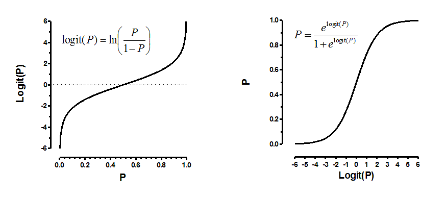
Logistic regression is an estimation of Logit function. Logit function is simply a log of odds in favor of the event. This function creates a s-shaped curve with the probability estimate, which is very similar to the required step wise function. Here goes the first definition :

Logit Function:

Logistic regression is an estimate of a logit function. Here is how the logit function looks like:👁 logit

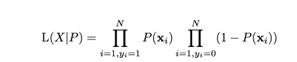
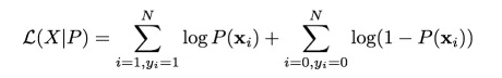
Now that you know what we are trying to estimate, next is the definition of the function we are trying to optimize to get the estimates of coefficient. This function is analogous to the square of error in linear regression and is known as the likelihood function. Here goes our next definition.

Likelihood Function

👁 likelihood function

Given the complicated derivative of the likelihood function, we consider a monotonic function which can replicate the likelihood function and simplify derivative. This is the log of likelihood function. Here goes the next definition.

Log Likelihood

👁 loglikelihood function

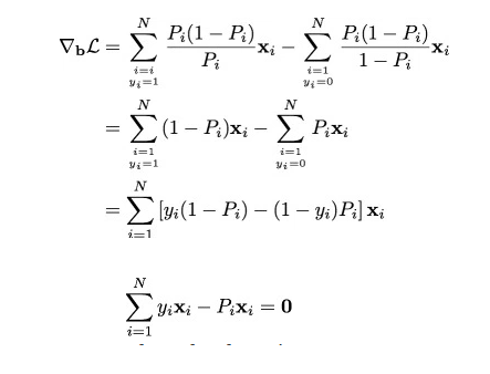
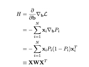
Finally we have the derivatives of log likelihood function. Following are the first and second derivative of log likelihood function.

Derivative of Likelihood Function

👁 first derivative

Hessian Matrix (second derivative)

👁 Hessian Matrix

Finally, we are looking to solve the following equation.

👁 equations

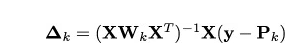
As we now have all the derivative, we will finally apply the Newton Raphson method to converge to optimal solution. Here is a recap of Newton Raphson method.

Newton Raphson Method

👁 nr

The Code

Here is a R code which can help you make your own logistic function

Let’s get our functions right.

#Calculate the first derivative of likelihood function given output (y) , input (x) and pi (estimated probability)
calculateder <- function(y,x,pi) {
derv <- y*x - pi*x
derv_sum <- sum(derv)
return(derv_sum)
}

#Calculate the likelihood function given output(y) and pi
calculatell <- function(y,pi) {
ll <- 1
ll_unit <- 1:length(y)
for (i in 1:length(y)){
ll_unit[i] <- ifelse(y[i] == 1,pi[i],1-pi[i])
ll = ll_unit[i]*ll
}
return(ll)
}

#Calculate the value of pi (predictions on each observation) given x_new(input) and estimated betas
findpi <- function(x_new,beta){
pi <- 1:nrow(x_new)
expon <- 1:nrow(x_new)
for (i in 1:nrow(x_new)){
expon[i] <- 0
for (j in 1:ncol(x_new)){
expo <- x_new[i,j] * beta[j]
expon[i] <- expo + expon[i]}
pi[i] <- exp(expon[i])/(1+exp(expon[i]))
}
return(pi)
}

#Calculate the matrix W with all diagnol values as pi 
findW <- function(pi){
W <- matrix(0,length(pi),length(pi))
for (i in 1:length(pi)){
W[i,i] <- pi[i]*(1-pi[i])
}
return(W)
}

# Lets now make the logistic function given list of required inputs
logistic <- function(x,y,vars,obs,learningrate,dif) {
beta <- rep(0, (vars+1))
bias <- rep(1, obs)
x_new <- cbind(bias,x)
derivative <- 1:(vars+1)
diff <- 10000
while(diff > dif) {
pi <- findpi(x_new,beta)
pi <- as.vector(pi)
W <- findW(pi)
derivative <- (solve(t(x_new)%*%W%*%as.matrix(x_new))) %*% (t(x_new)%*%(y - pi))
beta = beta + derivative
diff <- sum(derivative^2)
ll <- calculatell(y,pi)
print(ll)
}
return(beta)
}

# Time to test our algorithm with the values we mentioned at the start of the article
x <- 1:10
y <- c(rep(0, 4),1,0,1,0,1,1)
a <- logistic(x,y,1,10,0.01,0.000000001)
calculatell(y,findpi(x_new,a))
#Log Likelihood = 0.01343191
data <- cbind(x,y)
data <- as.data.frame(data)
mylogit <- glm(y ~ x, data = data, family = "binomial")
mylogit
preds <- predict(mylogit, newdata = data,type ="response")
calculatell(data$y,preds)
#Log Likelihood = 0.01343191
#Isn't this amazing!!!

End Notes

This might seem like a simple exercise, but I feel that this is extremely important before you start using Logistic as a black box. As an exercise you should try making these calculations using a gradient descent method. Also, for people conversant with Python, here is a small challenge to you – can you write a Python code for the larger community and share it in comments below?

Login to continue reading and enjoy expert-curated content.

Free Courses