VOOZH about

URL: https://www.analyticsvidhya.com/blog/2021/01/gaussian-naive-bayes-with-hyperpameter-tuning/

⇱ Naive Bayes | Gaussian Naive Bayes with Hyperpameter Tuning in Python


India's Most Futuristic AI Conference Is Back – Bigger, Sharper, Bolder

  • d
  • :
  • h
  • :
  • m
  • :
  • s

Reading list

Gaussian Naive Bayes with Hyperparameter Tuning

Akshay Last Updated : 27 Jan, 2021
6 min read

This article was published as a part of the Data Science Blogathon.

Introduction

Naive Bayes is a classification technique based on the Bayes theorem. It is a simple but powerful algorithm for predictive modeling under supervised learning algorithms. The technique behind Naive Bayes is easy to understand.  Naive Bayes has higher accuracy and speed when we have large data points.

There are three types of Naive Bayes models: Gaussian, Multinomial, and Bernoulli.

  1. Gaussian Naive Bayes – This is a variant of Naive Bayes which supports continuous values and has an assumption that each class is normally distributed. 
  2. Multinomial Naive Bayes – This is another variant which is an event-based model that has features as vectors where sample(feature) represents frequencies with which certain events have occurred.
  3. Bernoulli – This variant is also event-based where features are independent boolean which are in binary form.

Understanding Statistics behind Gaussian Naive Bayes

Gaussian Naive Bayes is based on Bayes’ Theorem and has a strong assumption that predictors should be independent of each other. For example, Should we give a Loan applicant would depend on the applicant’s income, age, previous loan, location, and transaction history? In real life scenario, it is most unlikely that data points don’t interact with each other but surprisingly Gaussian Naive Bayes performs well in that situation. Hence, this assumption is called class conditional independence.

Let’s understand with an example of 2 dice:

Gaussian Naive Bayes says that events should be mutually independent and to understand that let’s start with basic statistics.

  1. Event A -> Roll 1 on 1st Dice
  2. Event B -> Roll 1 on 2nd Dice

Let A and B be any events with probabilities P(A) and P(B). Both the events are mutually independent. So if we have to calculate the probability of both the events then:

  • P(A) = 1/6 and,
  • P(B) = 1/6
  • P(A and B) = P(A)P(B) = 1/36

If we are told that B has occurred, then the probability of A might change. The new probability of A is called the conditional probability of A given B.

Conditional Probability:

  • P(A|B) = 1/6
  • P(B|A) = 1/6

We can say that:

  • P(A|B) = P(A and B)/P(B) It can also be written as,
  • P(A|B) = P(A) or,
  • P(A and B) = P(A)P(B)

OR

  • Multiplication rule: P(A and B) = P(A|B) P(B) OR,
  • Multiplication rule: P(B and A) = P(B|A)P(A)

We can also write the equation as:

  • P(A|B) P(B) = P(B|A)P(A)

This gives us the Bayes theorem:

P(A|B) = P(B|A)P(A)/P(B)

  • P(A|B) is the posterior probability of class (A, target) given predictor (B, attributes).
  • P(A) is the prior probability of class.
  • P(B|A) is the probability of the predictor given class.
  • P(B) is the prior probability of the predictor.
  • Posterior Probability = (Conditional Probability x Prior probability)/ Evidence

Understanding how Algorithm works

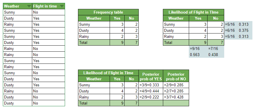
Let’s understand the working of Naive Bayes with an example. consider a use case where we want to predict if a flight would land in the time given weather conditions on that specific day using the Naive Bayes algorithm. Below are the steps which algorithm follows:

  1. Calculate prior probability for given class labels
  2. Create a frequency table out of given historical data
  3. Find likelihood probability with each attribute of each class. For example, given it was Sunny weather, was the flight in time.
  4. Now put these values into the Bayes formula and calculate posterior probability.
  5. The class with the highest probability will be the outcome.

Problem: Given the historical data, we want to predict if the flight will land in time if the weather is Dusty?

Probability of Flight arriving in time:

P(Yes | Dusty) = P( Dusty | Yes) * P(Yes) / P(Dusty)

1. Calculating Prior probability

P(Dusty) = 6/16 = 0.375

P(Yes)= 9/16 = 0.563

2. Calculating Posterior probability

P (Dusty | Yes) = 4/9 = 0.444

Putting Prior and Posterior in our equation:

P (Yes | Dusty) = 0.444 * 0.563 / 0.375 = 0.666

Probability of Flight not arriving in time:

P(No | Dusty) = P( Dusty | No) * P(No) / P(Dusty)

1. Calculating Prior probability

P(Dusty) = 6/16 = 0.375

P(No) = 7/16 = 0.438

2. Calculating Posterior probability

P(Dusty | No) = 2/7 = 0.285

Putting Prior and Posterior in our equation

P(No | Dusty) = 0.285*0.438 / 0.375 = 0.332

Given its Dusty weather flight will land in time. Here probability of flight arriving in time (0.666) is greater than flight not arriving in time (0.332), So the class assigned will be ‘In Time’.

Zero Probability Phenomena

Suppose we are predicting if a newly arrived email is spam or not. The algorithm predicts based on the keyword in the dataset. While analyzing the new keyword “money” for which there is no tuple in the dataset, in this scenario, the posterior probability will be zero and the model will assign 0 (Zero) probability because the occurrence of a particular keyword class is zero. This is referred to as “Zero Probability Phenomena”.

We can get over this issue by using smoothing techniques. One of the techniques is Laplace transformation, which adds 1 more tuple for each keyword class pair. In the above example, let’s say we have 1000 keywords in the training dataset. Where we have 0 tuples for keyword “money”, 990 tuples for keyword “password” and 10 tuples for keyword “account” for classifying an email as spam. Without Laplace transformation the probability will be: 0 (0/1000), 0.990 (990/1000) and 0.010 (10/1000).

Now if we apply Laplace transformation and add 1 more tuple for each keyword then the new probability will be 0.001 (1/1003), 0.988 (991/1003), and 0.01 (11/1003).

Pros and Cons

Pros

  • Simple, Fast in processing, and effective in predicting the class of test dataset. So you can use it to make real-time predictions for example to check if an email is a spam or not. Email services use this excellent algorithm to filter out spam emails.
  • Effective in solving a multiclass problem which makes it perfect for identifying Sentiment. Whether it belongs to the positive class or the negative class.
  • Does well with few samples for training when compared to other models like Logistic Regression.
  • Easy to obtain the estimated probability for a prediction. This can be obtained by calculating the mean, for example, print(result.mean()).
  • It performs well in case of text analytics problems.
  • It can be used for multiple class prediction problems where we have more than 2 classes.

Cons

  • Relies on and often an incorrect assumption of independent features. In real life, you will hardly find independent features. For example, Loan eligibility analysis would depend on the applicant’s income, age, previous loan, location, and transaction history which might be interdependent.
  • Not ideal for data sets with a large number of numerical attributes. If the number of attributes is larger then there will be high computation cost and it will suffer from the Curse of dimensionality.
  • If a category is not captured in the training set and appears in the test data set then the model is assign 0 (zero) probability which leads to incorrect calculation. This phenomenon is referred to as ‘Zero frequency’ and to overcome ‘Zero frequency’ phenomena you will have to use smoothing techniques.

Python Code

# Gaussian Naive Bayes Classification
import numpy as n
import pandas as p
from sklearn.model_selection import c
from sklearn.metrics import a, 
from sklearn.naive_bayes import G
from sklearn.model_selection import t,
import matplotlib.pyplot as p
import seaborn as S
.<a onclick="parent.postMessage({'referent':'.seaborn.set_style'}, '*')">set_style("whitegrid")
import W
.("ignore")
import scipy.stats as s
%matplotlib inline
 = .<a onclick="parent.postMessage({'referent':'.pandas.read_csv'}, '*')">read_csv('/kaggle/input/pima-indians-diabetes-database/diabetes.csv')
 = .(columns=['Outcome'],axis=1)
 = ['Outcome']
from sklearn.impute import S
 = (missing_values=0, strategy="mean")
 = .
 = .<a onclick="parent.postMessage({'referent':'.pandas.DataFrame'}, '*')">DataFrame(.())
 = .<a onclick="parent.postMessage({'referent':'.pandas.DataFrame'}, '*')">DataFrame(.())
.columns = 
.columns = 
.()
#Predicting train and test accuracy
 = .(, ).()
# Accuray Score on train dataset a
 = (,)
('accuracy_score on train dataset : ', )
# predict the target on the test dataset
 = .()
# Accuracy Score on test dataset
 = (,)
('accuracy_score on test dataset : ', )
#accuracy_score on train dataset : 0.7597765363128491
#accuracy_score on test dataset : 0.7575757575757576

Hyperparameter Tuning to improve Accuracy

.<a onclick="parent.postMessage({'referent':'.numpy.logspace'}, '*')">logspace(0,-9, num=10)
from sklearn.model_selection import R
 = (n_splits=5,  n_repeats=3, random_state=999)
from sklearn.preprocessing import P
 = {'var_smoothing': .<a onclick="parent.postMessage({'referent':'.numpy.logspace'}, '*')">logspace(0,-9, num=100)}

 = (estimator=, param_grid=p, cv=c,verbose=1,scoring='accuracy')
 = ().()
.(, );
 = .(.['params'])
['test_score'] = .['mean_test_score']
# predict the target on the test dataset
 = .()
# Accuracy Score on test dataset
 = (,)
('accuracy_score on test dataset : ', )
#accuracy_score on test dataset : 0.7922077922077922

The media shown in this article are not owned by Analytics Vidhya and is used at the Author’s discretion.

Login to continue reading and enjoy expert-curated content.

Free Courses

Exploratory Data Analysis with Python & GenAI

Learn EDA with Python: Transform data into insights using PandasAI & more.

Data Science Course

Build a powerful 2026-ready data science resume using AI tools.

No Code Predictive Analytics with Orange

No-code AI course for business pros with real-world ML use cases.

Adaptive Email Agents with DSPy

Build adaptive email agents with DSPy using context and smart learning.

Introduction to AI & ML

AI & ML are transforming industries. Learn their impacts in this course.

Responses From Readers

Chiranjeevi

Hey congrats Akshay, nice article 🙂

Flagship Programs

GenAI Pinnacle Program| GenAI Pinnacle Plus Program| AI/ML BlackBelt Program| Agentic AI Pioneer Program

Free Courses

Generative AI| DeepSeek| OpenAI Agent SDK| LLM Applications using Prompt Engineering| DeepSeek from Scratch| Stability.AI| SSM & MAMBA| RAG Systems using LlamaIndex| Building LLMs for Code| Python| Microsoft Excel| Machine Learning| Deep Learning| Mastering Multimodal RAG| Introduction to Transformer Model| Bagging & Boosting| Loan Prediction| Time Series Forecasting| Tableau| Business Analytics| Vibe Coding in Windsurf| Model Deployment using FastAPI| Building Data Analyst AI Agent| Getting started with OpenAI o3-mini| Introduction to Transformers and Attention Mechanisms

Popular Categories

AI Agents| Generative AI| Prompt Engineering| Generative AI Application| News| Technical Guides| AI Tools| Interview Preparation| Research Papers| Success Stories| Quiz| Use Cases| Listicles

Generative AI Tools and Techniques

GANs| VAEs| Transformers| StyleGAN| Pix2Pix| Autoencoders| GPT| BERT| Word2Vec| LSTM| Attention Mechanisms| Diffusion Models| LLMs| SLMs| Encoder Decoder Models| Prompt Engineering| LangChain| LlamaIndex| RAG| Fine-tuning| LangChain AI Agent| Multimodal Models| RNNs| DCGAN| ProGAN| Text-to-Image Models| DDPM| Document Question Answering| Imagen| T5 (Text-to-Text Transfer Transformer)| Seq2seq Models| WaveNet| Attention Is All You Need (Transformer Architecture) | WindSurf| Cursor

Popular GenAI Models

Llama 4| Llama 3.1| GPT 4.5| GPT 4.1| GPT 4o| o3-mini| Sora| DeepSeek R1| DeepSeek V3| Janus Pro| Veo 2| Gemini 2.5 Pro| Gemini 2.0| Gemma 3| Claude Sonnet 3.7| Claude 3.5 Sonnet| Phi 4| Phi 3.5| Mistral Small 3.1| Mistral NeMo| Mistral-7b| Bedrock| Vertex AI| Qwen QwQ 32B| Qwen 2| Qwen 2.5 VL| Qwen Chat| Grok 3

AI Development Frameworks

n8n| LangChain| Agent SDK| A2A by Google| SmolAgents| LangGraph| CrewAI| Agno| LangFlow| AutoGen| LlamaIndex| Swarm| AutoGPT

Data Science Tools and Techniques

Python| R| SQL| Jupyter Notebooks| TensorFlow| Scikit-learn| PyTorch| Tableau| Apache Spark| Matplotlib| Seaborn| Pandas| Hadoop| Docker| Git| Keras| Apache Kafka| AWS| NLP| Random Forest| Computer Vision| Data Visualization| Data Exploration| Big Data| Common Machine Learning Algorithms| Machine Learning| Google Data Science Agent
👁 Av Logo White

Continue your learning for FREE

Forgot your password?
👁 Av Logo White

Enter OTP sent to

Edit

Wrong OTP.

Enter the OTP

Resend OTP

Resend OTP in 45s

👁 Popup Banner
👁 AI Popup Banner