A Comprehensive Guide to Expectation-Maximization Algorithm

8 min read

Introduction

In many real-life machine learning scenarios, numerous relevant features are available for model building, but only a fraction of them are observable. Due to the absence of values for unobserved (latent) variables, the Expectation-Maximization (EM) algorithm leverages existing data to estimate optimal values for these variables and subsequently determine model parameters. EM iteratively computes expected values for latent variables based on observed data points and maximizes the likelihood function through parameter updates. This approach is particularly valuable in scenarios like clustering algorithms, such as K-means, where latent variables play a crucial role in defining cluster memberships and optimizing cluster centroids. By iteratively refining these latent variables, EM facilitates robust model estimation and enhances the performance of clustering algorithms.

Learning Objectives

• Understand the concept of latent variables and their role in machine learning models.
• Learn the principles and steps of the Expectation-Maximization (EM) algorithm.
• Explore the advantages and disadvantages of the EM algorithm in parameter estimation and missing data handling.
• Discover the applications of the EM algorithm in various domains such as natural language processing, image reconstruction, and model parameter estimation.
• Gain practical experience in implementing Gaussian Mixture Models (GMM) using the EM algorithm in Python.

This article was published as a part of the Data Science Blogathon

What is Expectation-Maximization (EM) algorithm?

A latent variable model consists of observable variables along with unobservable variables. Observed variables are those variables in the dataset that can be measured whereas unobserved (latent/hidden) variables are inferred from the observed variables.

• It can be used to find the local maximum likelihood (MLE) parameters or maximum a posteriori (MAP) parameters for latent variables in a statistical or mathematical model.
• It is used to predict these missing values in the dataset, provided we know the general form of probability distribution associated with these latent variables.
• In simple words, the basic idea behind this algorithm is to use the observable samples of latent variables to predict the values of samples that are unobservable for learning. This process is repeated until the convergence of the values occurs.

Detailed Explanation of the EM Algorithm

• Given a set of incomplete data, start with a set of initialized parameters.
• Expectation step (E – step): In this expectation step, by using the observed available data of the dataset, we can try to estimate or guess the values of the missing data. Finally, after this step, we get complete data having no missing values.
• Maximization step (M – step): Now, we have to use the complete data, which is prepared in the expectation step, and update the parameters.
• Repeat step 2 and step 3 until we converge to our solution.

Aim of Expectation-Maximization algorithm

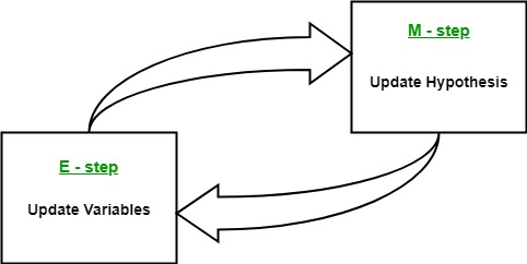
The Expectation-Maximization algorithm aims to use the available observed data of the dataset to estimate the missing data of the latent variables and then using that data to update the values of the parameters in the maximization step.

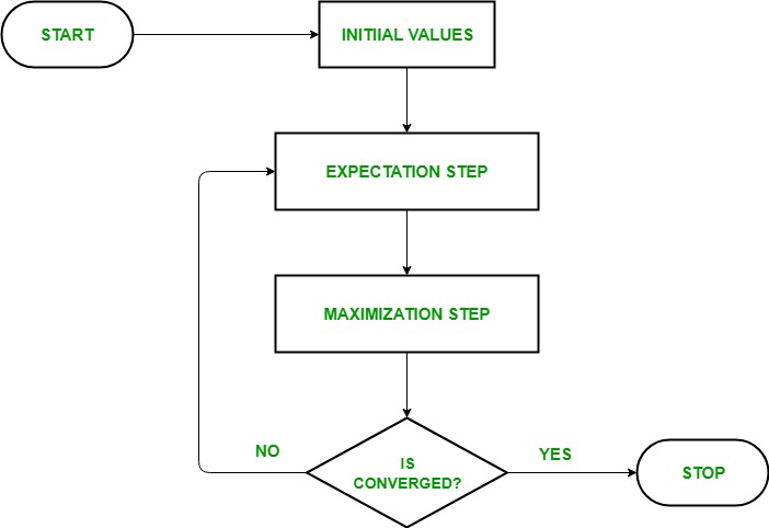
Let us understand the EM algorithm in a detailed manner:

• nitialization Step: In this step, we initialized the parameter values with a set of initial values, then give the set of incomplete observed data to the system with the assumption that the observed data comes from a specific model i.e, probability distribution.
• Expectation Step: In this step, by using the observed data to estimate or guess the values of the missing or incomplete data. It is used to update the variables.
• Maximization Step: In this step, we use the complete data generated in the “Expectation” step to update the values of the parameters i.e, update the hypothesis.
• Checking of convergence Step: Now, in this step, we checked whether the values are converging or not, if yes, then stop otherwise repeat these two steps i.e, the “Expectation” step and “Maximization” step until the convergence occurs.

Flow chart for EM algorithm

Advantages and Disadvantages of EM algorithm

• The basic two steps of the EM algorithm i.e, E-step and M-step are often pretty easy for many of the machine learning problems in terms of implementation.
• The solution to the M-steps often exists in the closed-form.
• It is always guaranteed that the value of likelihood will increase after each iteration.

• It has slow convergence.
• It converges to the local optimum only.
• It takes both forward and backward probabilities into account. This thing is in contrast to that of numerical optimization which considers only forward probabilities.

Applications of EM Algorithm

The latent variable model has several real-life applications in Machine learning:

• Used to calculate the Gaussian density of a function.
• Helpful to fill in the missing data during a sample.
• It finds plenty of use in different domains such as Natural Language Processing (NLP), Computer Vision, etc.
• Used in image reconstruction in the field of Medicine and Structural Engineering.
• Used for estimating the parameters of the Hidden Markov Model (HMM) and also for some other mixed models like Gaussian Mixture Models, etc.
• Used for finding the values of latent variables.

Use-Case of EM Algorithm

Basics of Gaussian Distribution

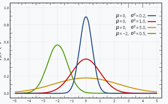
You’re likely familiar with Gaussian Distributions (or the Normal Distribution) since this distribution sees heavy use in the field of Machine Learning and Statistics. It has a bell-shaped curve, with the observations symmetrically distributed around the mean (average) value.

The given image shown has a few Gaussian distributions with different values of the mean (μ) and variance (σ²). Remember that the higher the σ (standard deviation) value more would be the spread along the axis.

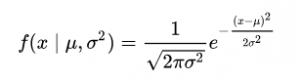
In 1-D space, the probability density function of a Gaussian distribution is given by:

Fig. Probability Density Function (PDF)where μ represents the mean and σ² represents the variance.

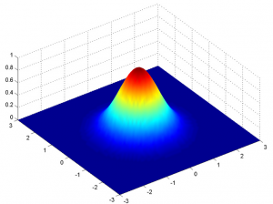
But this would only be true for a variable in 1-D only. In the case of two variables, we will have a 3D bell curve instead of a 2D bell-shaped curve as shown below:

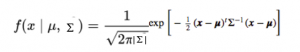
The probability density function would be given by:

where x is the input vector, μ is the 2-D mean vector, and Σ is the 2×2 covariance matrix.  We can generalize the same for the d-dimension.

Thus, for the Multivariate Gaussian model, we have x and μ as vectors of length d, and Σ would be a d x d covariance matrix.

Hence, for a dataset having d features, we would have a mixture of k Gaussian distributions (where k represents the number of clusters), each having a certain mean vector and variance matrix.

 

Gaussian Mixture Models

The main assumption of these mixture models is that there are a certain number of Gaussian distributions, and each of these distributions represents a cluster. Hence, a Gaussian Mixture model tries to group the observations belonging to a single distribution together.

Gaussian Mixture Models are probabilistic models which use the soft clustering approach for distributing the observations in different clusters i.e, different Gaussian distribution.

For Example, the Gaussian Mixture Model of 2 Gaussian distributions

We have two Gaussian distributions-  N(𝜇₁, 𝜎₁²) and N(𝜇₂, 𝜎₂²)

Here, we have to estimate a total of 5 parameters:

𝜃 = ( p, 𝜇₁, 𝜎₁²,𝜇₂, 𝜎₂²)

where p is the probability that the data comes from the first  Gaussian distribution and 1-p that it comes from the second Gaussian distribution. Then, the probability density function (PDF) of the mixture model is given by:

g(x|𝜃) = p g₁(x| 𝜇₁, 𝜎₁²) + (1-p)g₂(x| 𝜇₂, 𝜎₂² )

Objective: To best fit a given probability density by finding 𝜃 = ( p, 𝜇₁, 𝜎₁²,𝜇₂, 𝜎₂²) through EM iterations.

 Implementation of GMM in Python

Let’s delve into the code! In this implementation, we harness the power of the Sklearn Library in Python.

Using Sklearn, we leverage the GaussianMixture class, which seamlessly integrates the Expectation-Maximization (EM) algorithm for fitting a mixture of Gaussian models. After instantiating the object, we use the GaussianMixture.fit method to train the model and learn a Gaussian Mixture Model from the provided training data.

This implementation relies on fundamental concepts such as the EM algorithm and Gaussian Mixture Models, which play a crucial role in various machine learning algorithms and regression tasks. By understanding the underlying principles of these techniques and their application to random variables, we can effectively optimize the current parameters and enhance the performance of our models.

Step-1: Import necessary Packages and create an object of the Gaussian Mixture class

# Import necessary Packages
import numpy as np
import matplotlib.pyplot as plt
from sklearn.mixture import GaussianMixture

# Create an object of the Gaussian Mixture class
gmm = GaussianMixture(n_components = 2, tol=0.000001)

print(gmm)

Step-2: Fit the created object on the given dataset

gmm.fit(np.expand_dims(data, 1))

Step-3: Print the parameters of 2 input Gaussians

Gaussian_nr = 1
print('Input Normal_distb {:}: μ = {:.2}, σ = {:.2}'.format("1", Mean1, Standard_dev1))
print('Input Normal_distb {:}: μ = {:.2}, σ = {:.2}'.format("2", Mean2, Standard_dev2))

Input Normal_distb 1: μ = 2.0, σ = 4.0

Input Normal_distb 2: μ = 9.0, σ = 2.0

Step-4: Print the parameters after mixing of 2 Gaussians

for mu, sd, p in zip(gmm.means_.flatten(), np.sqrt(gmm.covariances_.flatten()), gmm.weights_):
 print('Normal_distb {:}: μ = {:.2}, σ = {:.2}, weight = {:.2}'.format(Gaussian_nr, mu, sd, p))
 g_s = stats.norm(mu, sd).pdf(x) * p
 plt.plot(x, g_s, label='gaussian sklearn');
 Gaussian_nr += 1

Normal_distb 1: μ = 1.7, σ = 3.8, weight = 0.61

Normal_distb 2: μ = 8.8, σ = 2.2, weight = 0.39

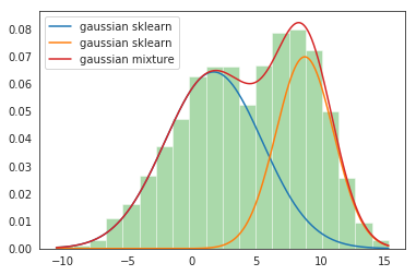
Step-5: Plot the distribution plots

sns.distplot(data, bins=20, kde=False, norm_hist=True)
gmm_sum = np.exp([gmm.score_samples(e.reshape(-1, 1)) for e in x]) 
plt.plot(x, gmm_sum, label='gaussian mixture');
plt.legend();

Conclusion

The Expectation-Maximization (EM) algorithm serves as a powerful tool for parameter estimation in models with latent variables and missing data. Despite its challenges, such as local optima and initialization dependence, EM remains widely used and versatile across various domains. This guide has provided an overview of EM principles, its applications in Gaussian Mixture Models, and its implementation using Python. By understanding EM’s concepts, practitioners can effectively leverage its capabilities for complex data analysis tasks, driving insights and advancements in the field of machine learning.

Key Takeaways

• Latent variables are unobservable variables that play a crucial role in modeling complex systems.
• The EM algorithm iteratively estimates latent variables and updates model parameters to maximize the likelihood of the observed data.
• EM algorithm advantages include versatility, handling missing data, and efficient computation, while disadvantages include local optima and slow convergence.
• EM algorithm finds applications in various fields like natural language processing, image processing, and model parameter estimation.
• Implementing Gaussian Mixture Models using the EM algorithm allows for flexible modeling of complex data distributions, enabling tasks such as clustering and density estimation.

Frequently Asked Questions

The media shown in this article on Expectation-Maximization Algorithm are not owned by Analytics Vidhya and is used at the Author’s discretion. 

Login to continue reading and enjoy expert-curated content.

Free Courses

Become an Author

Share insights, grow your voice, and inspire the data community.

• Reach a Global Audience
• Share Your Expertise with the World
• Build Your Brand & Audience

• Join a Thriving AI Community
• Level Up Your AI Game
• Expand Your Influence in Genrative AI

👁 imag