Demystifying the working of Principal Component Analysis!

This article was published as a part of the Data Science Blogathon.

Introduction

Principal Component Analysis (PCA) is one of the prominent dimensionality reduction techniques. It is valuable when we need to reduce the dimension of the dataset while retaining maximum information.

In this article, we will learn the need for PCA, PCA working, preprocessing steps required before applying PCA, and the interpretation of principal components.

Why do we need PCA?

PCA is not required unless you have a dataset with a large number of attributes. Generally, when we deal with real-world data we encounter a huge messy dataset with a large number of attributes.

If we apply any Machine Learning model on a huge dataset without reducing its dimensions then it would be computationally expensive.

Therefore, to reduce the dimension and to retain maximum information we need PCA as our objective is to deliver accurate ML models with less time and space complexity.

PCA is needed when dataset have large number of attributes. We can avoid PCA for smaller datasets.

Is there any preprocessing step required before applying PCA?

We need to keep the below points in  our mind before applying PCA

• PCA can not be applied to the dataset with null values. Hence, you need to treat null values before proceeding with PCA.   There are different ways of treating null values such as dropping the variables and imputing the missing data using mean or median.

• We shouldn’t apply PCA on the dataset having attributes on different scales. We need to standardize variables before applying PCA.

Let us take an example of Facebook Metric data set

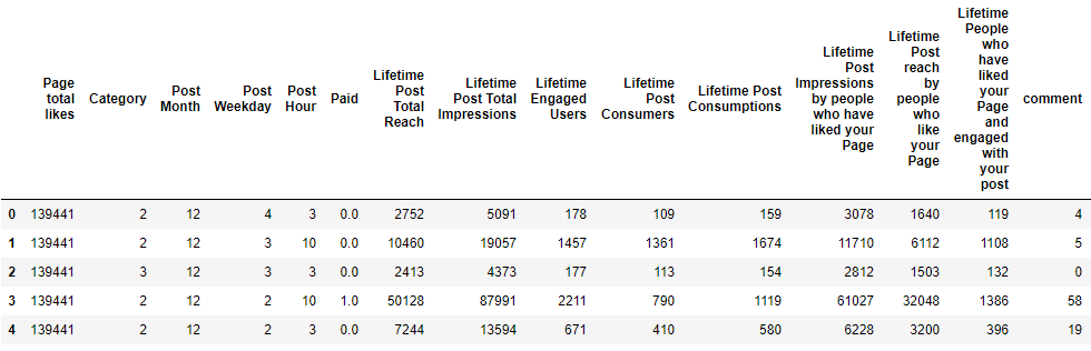
This dataset has 19 columns(or dimensions) and we will try to reduce its dimensions using PCA. Below you will find the python code and its output. We have dropped one categorical column for simplicity of analysis.

import pandas as pd
import numpy as np
import matplotlib.pyplot as plt
data = pd.read_csv(r"C:\Users\Himanshu\Downloads\Facebook_metrics\dataset_Facebook.csv",sep = ';')
data.drop(columns = 'Type',inplace = True) ##For simplicity we keep all data as numerical
data.head()

The output of the Facebook metrics dataset

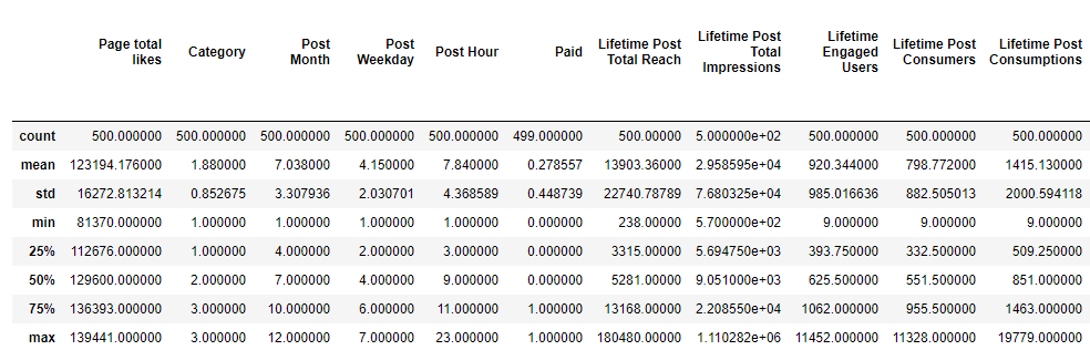
We will check the statistical summary of our dataset to find the scale of different attributes. Below we can see that every attribute is on a different scale. Therefore, we can not jump to PCA directly without changing the scales of attributes.

Statistical summary of data

We see that column “Post Weekday” has less variance and column “Lifetime Post Total Reach” has comparatively more variance.

Therefore, if we apply PCA without standardization of data then more weightage will be given to the “Lifetime Post Total Reach” column during the calculation of “eigenvectors” and “eigenvalues” and we will get biased principal components.

Now we will standardize the dataset using RobustScaler of sklearn library. Other ways of standardizing data are provided in sklearn like StandardScaler and MinMaxScaler and can be chosen as per the requirement.

from sklearn.preprocessing import RobustScaler
rs = RobustScaler()
scaled = pd.DataFrame(rs.fit_transform(data),columns = data.columns)
scaled.head()

Who decides the number of principal components?

Unless specified, the number of principal components will be equal to the number of attributes.

Our dataset has 18 attributes initially hence we get 18 principal components. These components are new variables which are in fact a linear combination of input variables.

Once we get the amount of variance explained by each principal component we can decide how many components we need for our model based on the amount of information we want to retain.

Principal components are uncorrelated with each other. These principal components are known as eigenvectors and the variances explained by each eigenvector is known as eigenvalues.

Below we have applied PCA on the scaled datasets. If we want a predefined number of components then we can do that it using PCA(n_components)

from sklearn.decomposition import PCA
scaled_data = scaled.dropna()
pca = PCA() ## If we need predefined number of components we can set n_components to any integer value
pca.fit_transform(scaled_data)
print(pca.explained_variance_ratio_)

Here the output is the variance explained by each principal component. We have 18 attributes in our dataset and hence we get 18 principal components.

Always remember that the first principal component will always hold maximum variance

You can observe the same in the output that the first principal component holds maximum variance followed by subsequent components.

Interpretation of Principal Component

Now we have 18 principal components and we will try to find out how these components are influenced by each attribute.

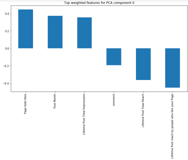
We can check the influence of the top 3 attributes (both positive and negative) for the first principal component.

Below is the python code to fetch the influence of attributes on principal components by changing the number of features and number of components.

def feature_weight(pca, n_comp, n_feat):
 #df = pd.DataFrame(np.round(pca.components_,2),columns = scaled_data.columns)
 comp = pd.DataFrame(np.round(pca.components_, 2), columns=scaled_data.keys()).iloc[n_comp - 1]
 comp.sort_values(ascending=False, inplace=True)
 comp = pd.concat([comp.head(n_feat), comp.tail(n_feat)])
 comp.plot(kind='bar', title='Top {} weighted attributes for PCA component {}'.format(n_feat, n_comp))
 plt.show()
 return comp
feature_weight(pca,0,3)

We can interpret here that our first principal component is mostly influenced by engagement to the post (like, comment, impression, and reach).

Likewise, we can interpret other principal components as per the understanding of data using the above plot.

Plot  to visualize variance by each principal component: Scree Plot

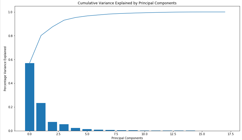
Below you can see a scree plot that depicts the variance explained by each principal component.

Here we can see that the top 8 components account for more than 95% variance. We can use these 8 principal components for our modelling purpose.

def screeplot(pca):
 var_len = len(pca.explained_variance_ratio_)
 indx = np.arange(var_len)
 var_pca = pca.explained_variance_ratio_
 plt.figure(figsize=(14, 8))
 ax = plt.subplot()
 cum_var = np.cumsum(var_pca)
 ax.bar(indx, var_pca)
 ax.plot(indx, cum_var)
 ax.set_xlabel("Principal Components")
 ax.set_ylabel("Percentage Variance Explained")
 plt.title('Cumulative Variance Explained by Principal Components')
screeplot(pca)

Finally, we reduce the number of attributes to 8 from the initial 18 attributes. We were also able to retain 95%  information of our dataset. Voila !! 🙂

Below is the scree plot for unscaled data just to check how different our principal components will be in the scaled version. We can see that there is a huge difference in principal components and the amount of variance explained. Here, the first component is explaining around 85% variance.

👁 Image

Similarly, you can check for each principal component how they have been influenced by attributes of unscaled data.

I hope this article would help to understand the basics of PCA.

If you like this article then I will share another article with basic mathematics about PCA.

The media shown in this article on Data Visualizations in Julia are not owned by Analytics Vidhya and is used at the Author’s discretion

Login to continue reading and enjoy expert-curated content.

Free Courses