Support Vector Machine and Principal Component Analysis Tutorial for Beginners

7 min read

This article was published as a part of the Data Science Blogathon

Introduction

A Support Vector Machine (SVM) is a very powerful and versatile Machine Learning model, capable of performing linear or nonlinear classification, regression, and even outlier detection. With this tutorial, we learn about the support vector machine technique and how to use it in scikit-learn. We will also discover the Principal Component Analysis and its implementation with scikit-learn.

1. Support Vector Machine

Another simple approach that any machine learning expert should know about is the support vector machine. Many people prefer the support vector machine because it produces great accuracy while using less computing power. SVM (Support Vector Machine) can be used for both regression and classification. However, it is widely applied in classifications objectives.

What is a Support Vector Machine?

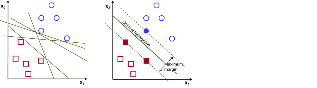
The objective of the support vector machine algorithm is to find a hyperplane in N-dimensional space(N — the number of features) that distinctly classifies the data points.

👁 svm and pca | svm

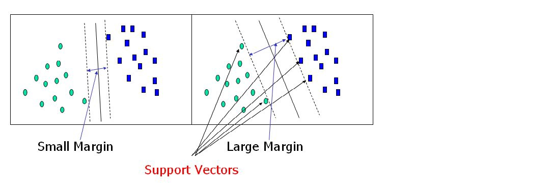
There are numerous hyper-planes from which to choose to split the two kinds of data points. Our goal is to discover a plane with the greatest margin, or the greatest distance between data points from both classes. Maximizing the margin distance adds some reinforcement, making it easier to classify future data points.

Hyper-planes and Support Vectors

👁 hyperplanes | svm and pca

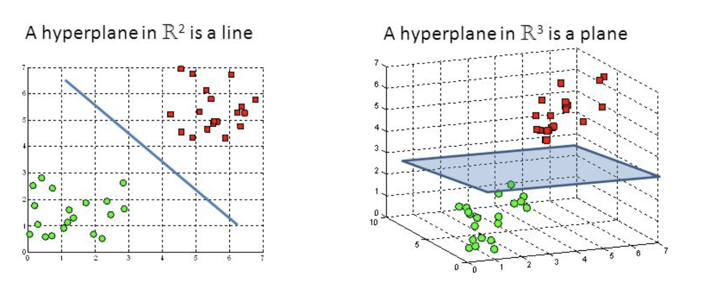
Hyper-planes are decision-making boundaries that help in data classification. Different classes can be assigned to data points on either side of the hyperplane. The hyperplane’s dimension is also determined by the number of features. If there are only two input characteristics, the hyperplane is simply a line. The hyperplane becomes a two-dimensional plane when the number of input features reaches three. When the number of features exceeds three, it becomes impossible to imagine.

👁 support vectors | svm and pca

Support vectors are data points that are closer to the hyperplane and have an influence on the hyperplane’s position and orientation. We increase the classifier’s margin by using these support vectors. The hyperplane’s position will be altered if the support vectors are deleted. These are the points that will assist us in constructing our SVM.

2. SVM Implementation in Python

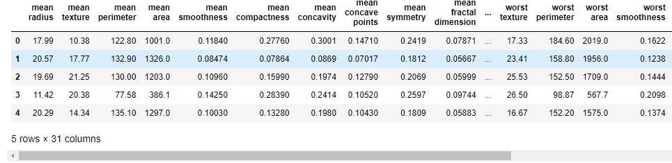
We will use a support vector machine in Predicting if the cancer diagnosis is benign or malignant based on several observations/features.

import pandas as pd
import numpy as np
import matplotlib.pyplot as plt
import seaborn as sns
%matplotlib inline
sns.set_style('whitegrid')

Python Code:

import pandas as pd
import numpy as np
from sklearn.datasets import load_breast_cancer
cancer = load_breast_cancer()
col_names = list(cancer.feature_names)
col_names.append('target')
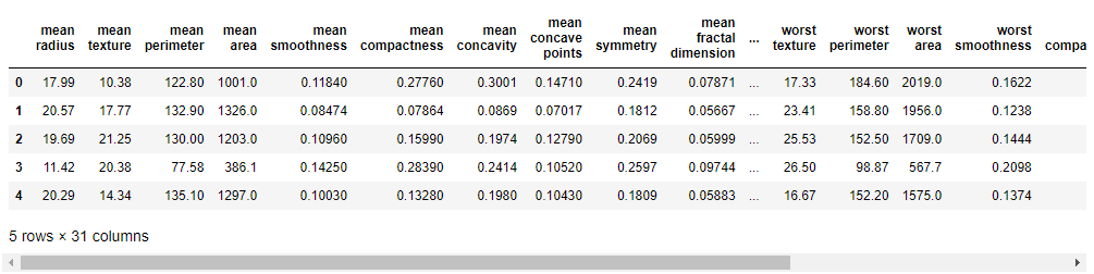
df = pd.DataFrame(np.c_[cancer.data, cancer.target], columns=col_names)
print(df.head())

👁 data

print(cancer.target_names)

👁 Image

df.describe()

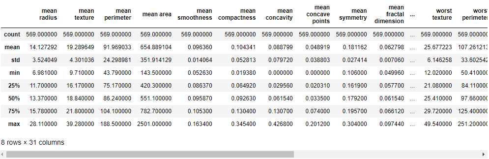
👁 data describe

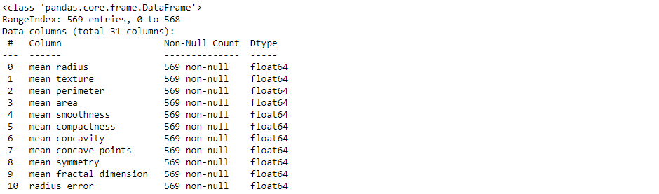
df.info()

👁 data info | svm and pca

Visualizing The Data

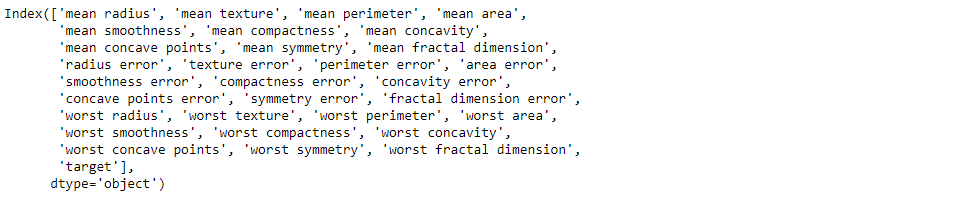
df.columns

👁 visualizing data | svm and pca

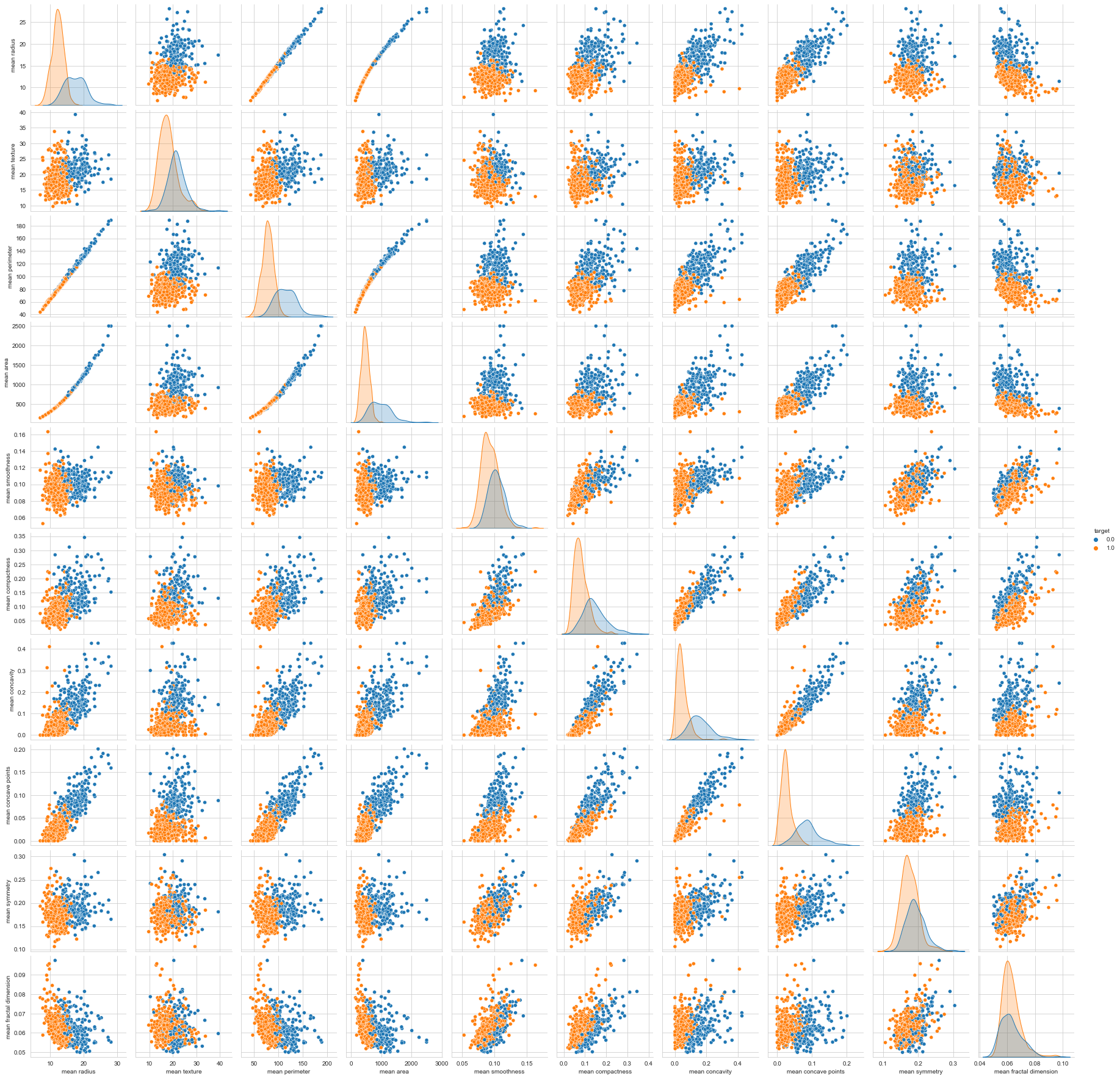
sns.pairplot(df, hue='target', vars=['mean radius', 'mean texture', 'mean perimeter', 'mean area', 
 'mean smoothness', 'mean compactness', 'mean concavity',
 'mean concave points', 'mean symmetry', 'mean fractal dimension'])

👁 data pairplot

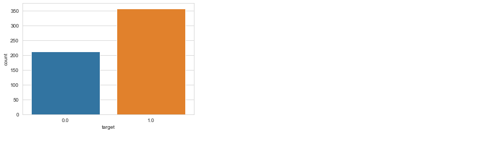
sns.countplot(df['target'], label = "Count")

👁 countplot

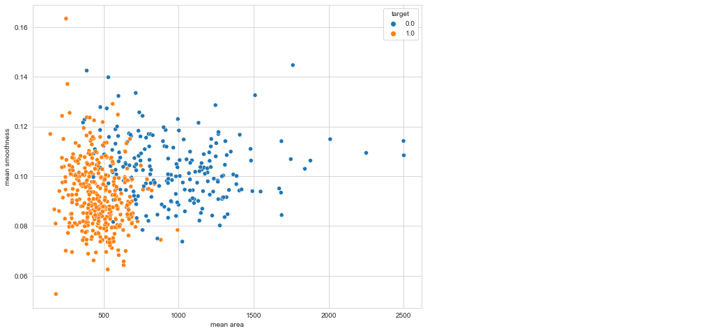
plt.figure(figsize=(10, 8))
sns.scatterplot(x = 'mean area', y = 'mean smoothness', hue = 'target', data = df)

👁 scatter plot | svm and pca

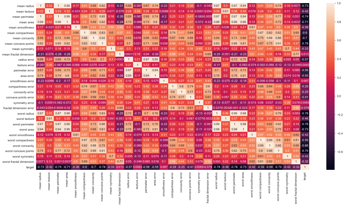
# Let's check the correlation between the variables 
# Strong correlation between the mean radius and mean perimeter, mean area and mean primeter
plt.figure(figsize=(20,10)) 
sns.heatmap(df.corr(), annot=True)

👁 corelation matrix | svm and pca

3. Model Training and finding problem solution

we use SVM sklearn for selection and for training, sklearn support vector machine to do  cross_val_score, train_test_split data.

from sklearn.model_selection import cross_val_score, train_test_split
from sklearn.pipeline import Pipeline
from sklearn.preprocessing import StandardScaler, MinMaxScaler
X = df.drop('target', axis=1)
y = df.target
print(f"'X' shape: {X.shape}")
print(f"'y' shape: {y.shape}")
pipeline = Pipeline([
 ('min_max_scaler', MinMaxScaler()),
 ('std_scaler', StandardScaler())
])
X_train, X_test, y_train, y_test = train_test_split(X, y, test_size=0.3, random_state=42)

👁 Image

from sklearn.metrics import accuracy_score, confusion_matrix, classification_report
def print_score(clf, X_train, y_train, X_test, y_test, train=True):
 if train:
 pred = clf.predict(X_train)
 clf_report = pd.DataFrame(classification_report(y_train, pred, output_dict=True))
 print("Train Result:n================================================")
 print(f"Accuracy Score: {accuracy_score(y_train, pred) * 100:.2f}%")
 print("_______________________________________________")
 print(f"CLASSIFICATION REPORT:n{clf_report}")
 print("_______________________________________________")
 print(f"Confusion Matrix: n {confusion_matrix(y_train, pred)}n")
 elif train==False:
 pred = clf.predict(X_test)
 clf_report = pd.DataFrame(classification_report(y_test, pred, output_dict=True))
 print("Test Result:n================================================") 
 print(f"Accuracy Score: {accuracy_score(y_test, pred) * 100:.2f}%")
 print("_______________________________________________")
 print(f"CLASSIFICATION REPORT:n{clf_report}")
 print("_______________________________________________")
 print(f"Confusion Matrix: n {confusion_matrix(y_test, pred)}n")

Support Vector Machines (Kernels)

Grid search is a popular way to find the right hyper-parameter values. Performing a large grid search first, then a refined grid search centred on the best results is frequently faster. Knowing what each hyper-parameter does can also help you identify the right part of the hyper-parameter space to search for.

SVM Kernel type:

1. Linear Kernel SVM

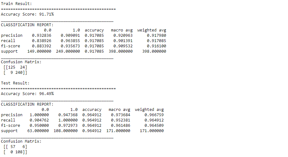
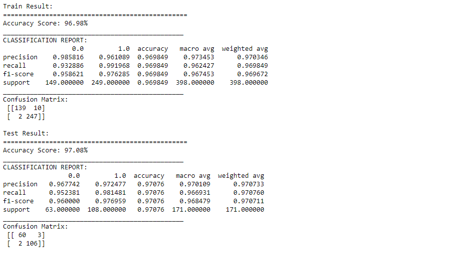
from sklearn.svm import LinearSVC
model = LinearSVC(loss='hinge', dual=True)
model.fit(X_train, y_train)
print_score(model, X_train, y_train, X_test, y_test, train=True)
print_score(model, X_train, y_train, X_test, y_test, train=False)

👁 train result | svm and pca

2. Polynomial Kernel SVM

This code trains an SVM classifier using a 2nd-degree polynomial kernel.

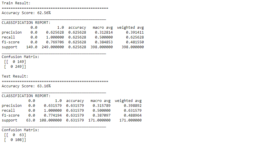
from sklearn.svm import SVC
# The hyperparameter coef0 controls how much the model is influenced by high degree ploynomials
model = SVC(kernel='poly', degree=2, gamma='auto', coef0=1, C=5)
model.fit(X_train, y_train)
print_score(model, X_train, y_train, X_test, y_test, train=True)
print_score(model, X_train, y_train, X_test, y_test, train=False)

👁 polynomial kernel svm | svm and pca

3. Radial Kernel SVM

Just like the polynomial features method, the similarity features can be useful with any

model = SVC(kernel='rbf', gamma=0.5, C=0.1)
model.fit(X_train, y_train)
print_score(model, X_train, y_train, X_test, y_test, train=True)
print_score(model, X_train, y_train, X_test, y_test, train=False)

👁 Train with radial kernel | svm and pca

Other kernels are available, but they are used far less frequently. Some kernels, for example, are specialized to particular data structures. When identifying text documents based on DNA sequences, string kernels are sometimes used.

How do you determine which kernel to use when there are so many options? If the training set is big or has a lot of characteristics, you should always attempt the linear kernel first. You should also try the Gaussian RBF kernel if the training set isn’t too big.

Support Vector Machine Hyper-parameter tuning

from sklearn.model_selection import GridSearchCV
param_grid = {'C': [0.01, 0.1, 0.5, 1, 10, 100], 
 'gamma': [1, 0.75, 0.5, 0.25, 0.1, 0.01, 0.001], 
 'kernel': ['rbf', 'poly', 'linear']} 
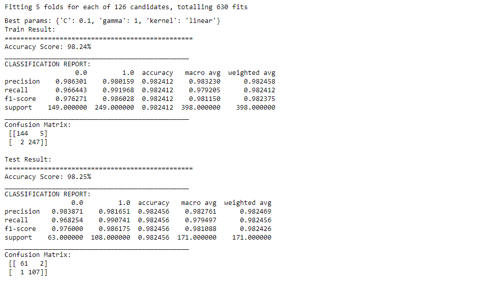
grid = GridSearchCV(SVC(), param_grid, refit=True, verbose=1, cv=5, iid=True)
grid.fit(X_train, y_train)
best_params = grid.best_params_
print(f"Best params: {best_params}")
svm_clf = SVC(**best_params)
svm_clf.fit(X_train, y_train)
print_score(svm_clf, X_train, y_train, X_test, y_test, train=True)
print_score(svm_clf, X_train, y_train, X_test, y_test, train=False)

👁 hyper parameter tuning svm

4. Principal Component Analysis

• Singular Value Decomposition is used to reduce the data’s dimensionality and project it to a lower-dimensional environment.
• Unsupervised Machine Learning
• A transformation of your data and attempts to find out what features explain the most variance in your data. For example:

👁 svm and pca | pca

robpca

.()

👁 data pca

PCA Visualization

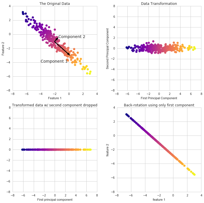
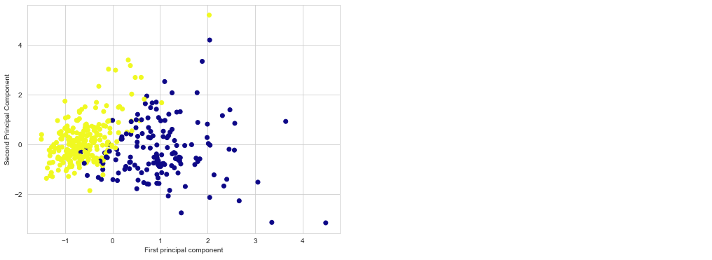
Because it’s difficult to represent high-dimensional data using a single scatter-plot, we may use PCA to determine the first two main components and visualize the data in this new, two-dimensional space. However, we must first scale our data to ensure that each feature has single unit variance.

scaler = StandardScaler()
X_train, X_test, y_train, y_test = train_test_split(X, y, test_size=0.3, random_state=42)
X_train = scaler.fit_transform(X_train)
X_test = scaler.transform(X_test)

PCA in Scikit Learn works in a similar way to the other preprocessing methods in Scikit Learn. We create a PCA object, use the fit method to discover the principle components, and then use transform to rotate and reduce the dimensionality.

When building the PCA object, we can additionally indicate how many components we wish to create.

from sklearn.decomposition import PCA
pca = PCA(n_components=3)
scaler = StandardScaler()
X_train = pca.fit_transform(X_train)
X_test = pca.transform(X_test)
X_train = scaler.fit_transform(X_train)
X_test = scaler.transform(X_test)

plt.figure(figsize=(8,6))
plt.scatter(X_train[:,0],X_train[:,1],c=y_train,cmap='plasma')
plt.xlabel('First principal component')
plt.ylabel('Second Principal Component')

👁 pca visualization

Using these two components we can easily separate these two classes.

Interpreting the components

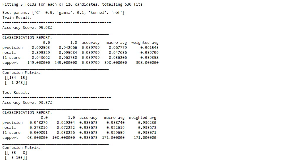
param_grid = {'C': [0.01, 0.1, 0.5, 1, 10, 100], 
 'gamma': [1, 0.75, 0.5, 0.25, 0.1, 0.01, 0.001], 
 'kernel': ['rbf', 'poly', 'linear']} 
grid = GridSearchCV(SVC(), param_grid, refit=True, verbose=1, cv=5, iid=True)
grid.fit(X_train, y_train)
best_params = grid.best_params_
print(f"Best params: {best_params}")
svm_clf = SVC(**best_params)
svm_clf.fit(X_train, y_train)
print_score(svm_clf, X_train, y_train, X_test, y_test, train=True)
print_score(svm_clf, X_train, y_train, X_test, y_test, train=False)

👁 result after pca | svm and pca

5. Summary

• What is a support vector machine?.
• Support vector machine implementation in Python.
• Support Vector Machine kernels (Linear, Polynomial, Radial).
• How to prepare the data for support vector machine algorithm.
• Support vector machine hyper-parameter tuning.
• How to utilize Principal Component Analysis to reduce the complexity of a problem.
• In sci-kit-learn, how to calculate the Principal Component Analysis for reuse on more data.

EndNote

Thank you for reading!
I hope you enjoyed the article and increased your knowledge.
Please feel free to contact me on Email
Something not mentioned or want to share your thoughts? Feel free to comment below And I’ll get back to you.

About the Author

Hardikkumar M. Dhaduk
Data Analyst | Digital Data Analysis Specialist | Data Science Learner
Connect with me on Linkedin
Connect with me on Github

The media shown in this article are not owned by Analytics Vidhya and are used at the Author’s discretion.

Login to continue reading and enjoy expert-curated content.

Free Courses

Become an Author

Share insights, grow your voice, and inspire the data community.

• Reach a Global Audience
• Share Your Expertise with the World
• Build Your Brand & Audience

• Join a Thriving AI Community
• Level Up Your AI Game
• Expand Your Influence in Genrative AI

👁 imag