Introduction to AdaBoost for Absolute Beginners

This article was published as a part of the Data Science Blogathon.

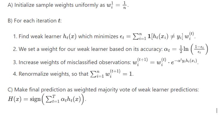
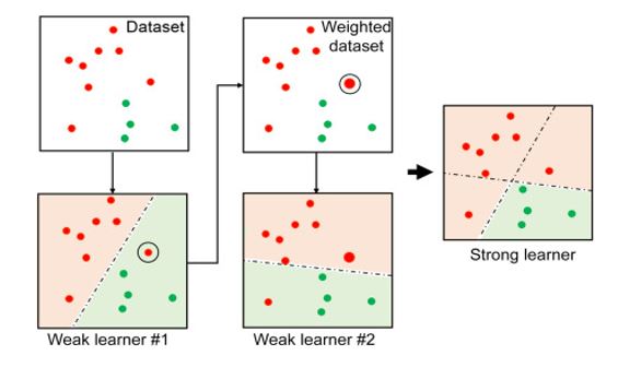
AdaBoost stands for Adaptive Boosting. It is a statistical classification algorithm. It is an algorithm that forms a committee of weak classifiers. It boosts the performance of machine learning algorithms. It helps you form a committee of weak classifiers by combining them into a single strong classifier. It can be used to solve a wide range of problems. The main idea of AdaBoost classifier is to increase the weight of the unclassified points and also to decrease the weight of the classified points. In the case of the Adaboost classifier, the trees are not fully grown, and the trees are just one root and two leaves, called stumps. The algorithm is as follows:

Adaboost model output

Advantages

• It is less prone to overfitting
• Less parameters tweaking
• Helps in reducing bias and variance
• Accuracy of weak classifiers can be improved using this method
• Easy to use

Disadvantages

• It needs a quality dataset
• Very sensitive to outliers and noise
• Slower than XGBoost
• Hyperparameter optimization is much more difficult

Implementation

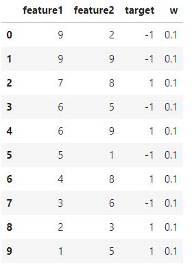
Creating a dataframe

First we will be creating a dataframe for whic we have to perform classification

df = pd.DataFrame()
df['feature1'] = [9,9,7,6,6,5,4,3,2,1]
df['feature2'] = [2,9,8,5,9,1,8,6,3,5]
df['target'] =[-1,-1,1,-1,1,-1,1,-1,1,1]
df['w'] = 1/df.shape[0]
df

Separate the features and target variable

#features and target values
X = df.iloc[:,0:2].values
y = df.iloc[:,2].values

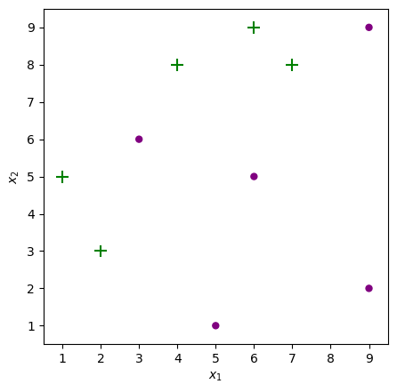
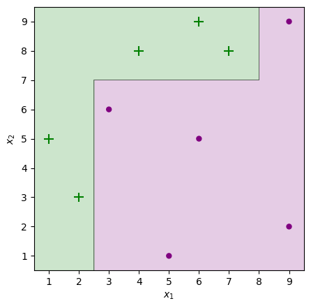
Plot the points in 2D Space

from typing import Optional
import numpy as np
import matplotlib.pyplot as plt
import matplotlib as mpl
#visualizing our datapoints
def plot_adaboost(X: np.ndarray,
 y: np.ndarray,
 clf=None,
 sample_weights: Optional[np.ndarray] = None,
 annotate: bool = False,
 ax: Optional[mpl.axes.Axes] = None) -> None:
 assert set(y) == {-1, 1}, 'Expecting response labels to be ±1'
 if not ax:
 fig, ax = plt.subplots(figsize=(5, 5), dpi=100)
 fig.set_facecolor('white')
 pad = 1
 x_min, x_max = X[:, 0].min() - pad, X[:, 0].max() + pad
 y_min, y_max = X[:, 1].min() - pad, X[:, 1].max() + pad
 if sample_weights is not None:
 sizes = np.array(sample_weights) * X.shape[0] * 100
 else:
 sizes = np.ones(shape=X.shape[0]) * 100
 X_pos = X[y == 1]
 sizes_pos = sizes[y == 1]
 ax.scatter(*X_pos.T, s=sizes_pos, marker='+', color='green')
 X_neg = X[y == -1]
 sizes_neg = sizes[y == -1]
 ax.scatter(*X_neg.T, s=sizes_neg, marker='.', c='purple')
 if clf:
 plot_step = 0.01
 xx, yy = np.meshgrid(np.arange(x_min, x_max, plot_step),
 np.arange(y_min, y_max, plot_step))
 Z = clf.predict(np.c_[xx.ravel(), yy.ravel()])
 Z = Z.reshape(xx.shape)
 
 if list(np.unique(Z)) == [1]:
 fill_colors = ['g']
 else:
 fill_colors = ['purple', 'g']
 ax.contourf(xx, yy, Z, colors=fill_colors, alpha=0.2)
 if annotate:
 for i, (x, y) in enumerate(X):
 offset = 0.05
 ax.annotate(f'$x_{i + 1}$', (x + offset, y - offset))
 ax.set_xlim(x_min+0.5, x_max-0.5)
 ax.set_ylim(y_min+0.5, y_max-0.5)
 ax.set_xlabel('$x_1$')
 ax.set_ylabel('$x_2$')
plot_adaboost(X, y)

Create a class AdaBoost with variables like stumps, errors etc.

class AdaBoost:
 def __init__(self):
 self.stumps = None
 self.stump_weights = None
 self.errors = None
 self.sample_weights = None

 def _check_X_y(self, X, y):
 assert set(y) == {-1, 1}, 'Response variable must be ±1'
 return X, y

Here we used Decision tree with max depth=1 as
our base classifier. AdaBoost repeatedly calls this weak learner with each time feeding it a different distribution of the training data. Every time we call, it generates a weak classifier and combine all of them into a single classifier which will give better performance.

from sklearn.tree import DecisionTreeClassifier
def fit(self, X: np.ndarray, y: np.ndarray, iters: int):
 X, y = self._check_X_y(X, y)
 n = X.shape[0]
 self.sample_weights = np.zeros(shape=(iters, n))
 self.stumps = np.zeros(shape=iters, dtype=object)
 self.stump_weights = np.zeros(shape=iters)
 self.errors = np.zeros(shape=iters)
 self.sample_weights[0] = np.ones(shape=n) / n
 for t in range(iters):
 curr_sample_weights = self.sample_weights[t]
 stump = DecisionTreeClassifier(max_depth=1, max_leaf_nodes=2)
 stump = stump.fit(X, y, sample_weight=curr_sample_weights)
 stump_pred = stump.predict(X)
 err = curr_sample_weights[(stump_pred != y)].sum()# / n
 stump_weight = np.log((1 - err) / err) / 2
 new_sample_weights = (curr_sample_weights * np.exp(-stump_weight * y * stump_pred))
 new_sample_weights /= new_sample_weights.sum()
 if t+1 < iters:
 self.sample_weights[t+1] = new_sample_weights
 self.stumps[t] = stump
 self.stump_weights[t] = stump_weight
 self.errors[t] = err
 return self
def predict(self, X):
 stump_preds = np.array([stump.predict(X) for stump in self.stumps])
 return np.sign(np.dot(self.stump_weights, stump_preds))
AdaBoost.fit = fit
AdaBoost.predict = predict
clf = AdaBoost().fit(X, y, iters=10)
plot_adaboost(X, y, clf)

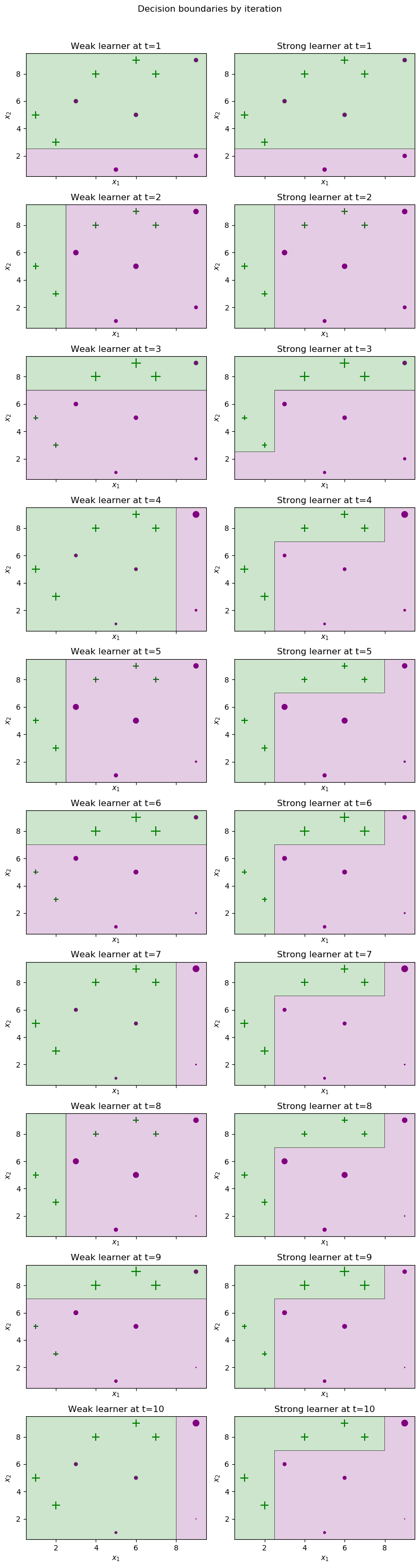
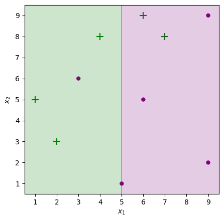
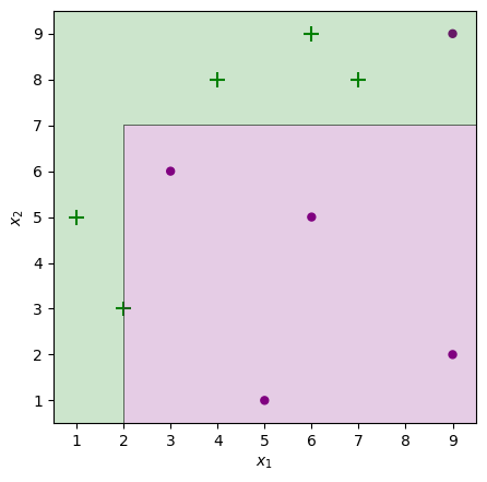
Visualizing our learner step by step

Here, the left column depicts the weak learner selected and the right column depicts the cumulative strong learner so far obtained in each iteration. Accordinh to the Adaboost classifier, the points which are misclassified in their previous iteration will be now more heavily weighted and therefore appear larger in the next iteration.

def truncate_adaboost(clf, t: int):
 assert t > 0, 't must be a positive integer'
 from copy import deepcopy
 new_clf = deepcopy(clf)
 new_clf.stumps = clf.stumps[:t]
 new_clf.stump_weights = clf.stump_weights[:t]
 return new_clf

def plot_staged_adaboost(X, y, clf, iters=10):
 fig, axes = plt.subplots(figsize=(8, iters*3),
 nrows=iters,
 ncols=2,
 sharex=True,
 dpi=100)
 fig.set_facecolor('white')
 _ = fig.suptitle('Decision boundaries by iteration')
 for i in range(iters):
 ax1, ax2 = axes[i]
 _ = ax1.set_title(f'Weak learner at t={i + 1}')
 plot_adaboost(X, y, clf.stumps[i],
 sample_weights=clf.sample_weights[i],
 annotate=False, ax=ax1)
 trunc_clf = truncate_adaboost(clf, t=i + 1)
 _ = ax2.set_title(f'Strong learner at t={i + 1}')
 plot_adaboost(X, y, trunc_clf,
 sample_weights=clf.sample_weights[i],
 annotate=False, ax=ax2)
 plt.tight_layout()
 plt.subplots_adjust(top=0.95)
 plt.show()
clf = AdaBoost().fit(X, y, iters=10)
plot_staged_adaboost(X, y, clf)

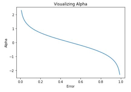
Plot for error rate is as follows-

The error rate is:

Comparison with sklearn’s inbuilt adaboost classifier

The n_estimators used are 1, 5, 10 trees to help notice a difference in performance and understand the working of boosting models.

Split the dataset into 70:30

from sklearn.model_selection import train_test_split
X_train, X_test, y_train, y_test = train_test_split(X, y, test_size=0.3)

Adaboost classifier with n_estimators=1

from sklearn.ensemble import AdaBoostClassifier
from sklearn import metrics
abc = AdaBoostClassifier(n_estimators=1,learning_rate=1)
model = abc.fit(X_train, y_train)
y_pred = model.predict(X_test)
plot_adaboost(X, y, model)

Adaboost classifier with n_estimators=5

from sklearn.ensemble import AdaBoostClassifier
from sklearn import metrics
abc = AdaBoostClassifier(n_estimators=5,learning_rate=1)
model = abc.fit(X_train, y_train)
y_pred = model.predict(X_test)
plot_adaboost(X, y, model)

Adaboost classifier with n_estimators=10

from sklearn.ensemble import AdaBoostClassifier
from sklearn import metrics
abc = AdaBoostClassifier(n_estimators=10,learning_rate=1)
model = abc.fit(X_train, y_train)
y_pred = model.predict(X_test)
plot_adaboost(X, y, model)

Conclusion

• Decisions trees are used as base classifiers
• Even though we have used weak classifiers still, all the instances are correctly classified.
• The main principle in the classifier is to increase the weight of misclassified datapoints and to decrease the weight value of correctly classified points. This updating of weights in the classifier allows the next iteration’s weak learner to have a meaningful decision boundary.
• When the trees are increased, the model results in better and more accurate classification.

The media shown in this article is not owned by Analytics Vidhya and are used at the Author’s discretion.

Login to continue reading and enjoy expert-curated content.

Free Courses