Let’s Find Out How to Make Engaging Videos?

This article was published as a part of the Data Science Blogathon.

Introduction

In this article, we will be predicting how engaging a video can be at the user level. We have been provided with a dataset that contains that user’s earlier videos engagement score along with their personal information.

We will build multiple regression models and see which one performs better.

Contents

1. Understanding Data
2. Industrial Applications
3. Exploratory Data Analysis
4. Feature Engineering
5. Model Building
6. Model Performance
7. Code
8. Conclusion

Understanding Data

This data was provided in a “Job-a-thon” contest organized at Analytics Vidya in February 2022. This data was available to those members who have participated in the contest. Since I have participated in the contest I was able to download the dataset. Here I will be presenting my approach to solving the problem.

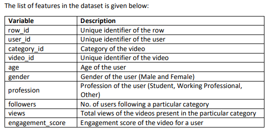
Features

Here age, gender, and profession are the user information provided to us and engagement_score represents how engaging their video was based on the scale of 1 to 5.

We are not allowed to use the row_id as a feature or build the new features using the row_id.

Industrial Applications

This problem is a day-to-day problem in today’s digital world.

Exploratory Data Analysis

user_id, category_id, and video_id are the categorical features in the dataset even though they are represented in numerical form.

Number of Unique Users in the data

df['user_id'].nunique()

Output : 27734

There are 27734 users in the given data.

Shape of Data

df.shape

Output : (89197, 10)

There are around 90,000 rows in the data and 10 columns including the target column.

Distribution of Numerical Features

num_features=['age','followers','views']
cat_features=['user_id','category_id','video_id','gender','profession']

df[num_features].hist(figsize=(10,10));

👁 Image

Source: Author

We can observe that there are mostly young users in the dataset. The age group between 15 to 25 is at its peak.

Distribution of Categorical Features

There is not much that we can get from user_id, category_id, and video_id. Let’s see the distribution of the ‘gender’ and ‘profession’.

sns.catplot(data=df[cat_features],kind='count',x='profession');

👁 Image

Source: Author

sns.catplot(data=df[cat_features],kind='count',x='gender');

👁 Image

Source: Author

We can observe that there is more number of video entries by ‘Male‘ users and ‘Students‘ is the most frequent profession and ‘Working Professionals’ are least active as per the given data.

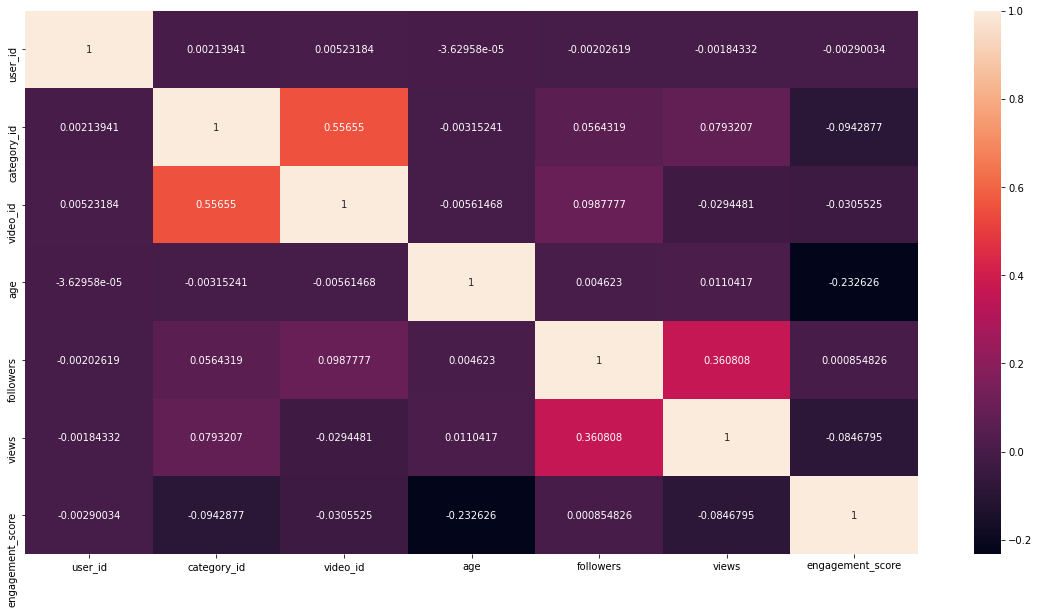
Feature Correlation

plt.figure(figsize=(20,10))
sns.heatmap(df.corr(),fmt='g',annot=True)

Source: Author

We can observe that there are two pair of features that shows some correlation. video_id, category_id and views, followers.

But there is no feature that shows a strong correlation with engament_score.

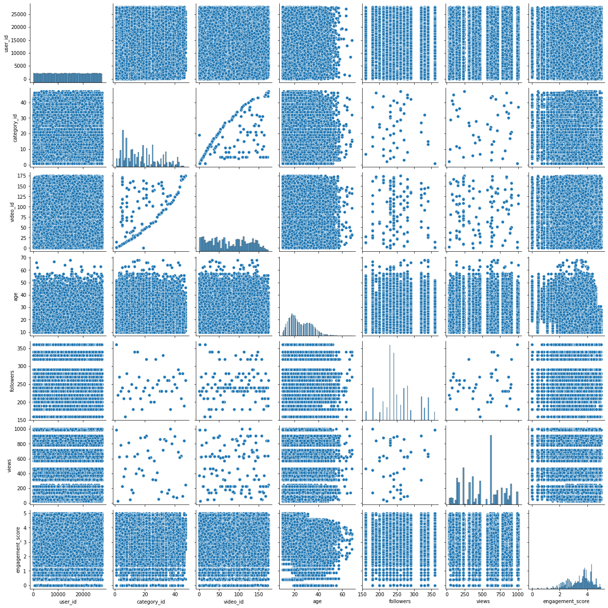
Pair Plot

sns.pairplot(df)

Source: Author

Pair plots also confirm the same that there is no strong correlation of engagement_score with any given feature.

Let’s see if we can build features that have a better correlation with the target (engagemnet_score) and help build a better predictive model.

Feature Engineering

We will try to create features using the followers, view, and engagement_score. We will find out how many min, mean, and max views and followers a user has. We will also find out min, mean, and max views and followers per category.

We will also build the features similarly using engagement_score. This will give us the min, max, and mean engagement_score of user and user per category.

First, let’s split the data into train and test datasets.

Splitting the dataset into train and test data

We are splitting the data into 80-20 split. 80% of the data will be used for training and 20% of the data will be used for testing.

features=['user_id', 'category_id', 'video_id', 'age', 'gender', 'profession',
 'followers', 'views']
target=['engagement_score']
x_train,x_test,y_train,y_test=train_test_split(df[features],df[target],test_size=0.2,random_state=42)
df_train=pd.concat([x_train,y_train],axis=1)
df_test=pd.concat([x_test,y_test],axis=1)

Building Features using ‘followers’ and ‘views’

grp_by=['user_id']
user_id_features=df_train.groupby(grp_by)['followers'].min().reset_index()
user_id_features.rename(columns={'followers':'min_followers'},inplace=True)
user_id_features['avg_followers']=df_train.groupby(grp_by)['followers'].mean().reset_index()['followers']
user_id_features['max_followers']=df_train.groupby(grp_by)['followers'].max().reset_index()['followers']
user_id_features['sum_followers']=df_train.groupby(grp_by)['followers'].sum().reset_index()['followers']
user_id_features['min_views']=df_train.groupby(grp_by)['views'].min().reset_index()['views']
user_id_features['mean_views']=df_train.groupby(grp_by)['views'].mean().reset_index()['views']
user_id_features['max_views']=df_train.groupby(grp_by)['views'].max().reset_index()['views']
user_id_features['sum_views']=df_train.groupby(grp_by)['views'].sum().reset_index()['views']
grp_by1=['user_id','category_id']
user_id_features1=df_train.groupby(grp_by1)['followers'].min().reset_index()
user_id_features1.rename(columns={'followers':'min_followers_category'},inplace=True)
user_id_features1['avg_followers_category']=df_train.groupby(grp_by1)['followers'].mean().reset_index()['followers']
user_id_features1['max_followers_category']=df_train.groupby(grp_by1)['followers'].max().reset_index()['followers']
user_id_features1['sum_followers_category']=df_train.groupby(grp_by1)['followers'].sum().reset_index()['followers']
user_id_features1['min_views_category']=df_train.groupby(grp_by1)['views'].min().reset_index()['views']
user_id_features1['mean_views_category']=df_train.groupby(grp_by1)['views'].mean().reset_index()['views']
user_id_features1['max_views_category']=df_train.groupby(grp_by1)['views'].max().reset_index()['views']
user_id_features1['sum_views_category']=df_train.groupby(grp_by1)['views'].sum().reset_index()['views']
df_train=pd.merge(df_train,user_id_features,how='left',on=grp_by)
df_test=pd.merge(df_test,user_id_features,how='left',on=grp_by)
df_train=pd.merge(df_train,user_id_features1,how='left',on=grp_by1)
df_test=pd.merge(df_test,user_id_features1,how='left',on=grp_by1)

Building Features using ‘engagement_score’

grp_by=['user_id']
user_id_features2=df_train.groupby(grp_by)['engagement_score'].min().reset_index()
user_id_features2.rename(columns={'engagement_score':'min_eng_score'},inplace=True)
user_id_features2['avg_eng_score']=df_train.groupby(grp_by)['engagement_score'].mean().reset_index()['engagement_score']
user_id_features2['max_eng_score']=df_train.groupby(grp_by)['engagement_score'].max().reset_index()['engagement_score']
user_id_features2['sum_eng_score']=df_train.groupby(grp_by)['engagement_score'].sum().reset_index()['engagement_score']
grp_by1=['user_id','category_id']
user_id_features3=df_train.groupby(grp_by1)['engagement_score'].min().reset_index()
user_id_features3.rename(columns={'engagement_score':'min_eng_score_category'},inplace=True)
user_id_features3['avg_eng_score_category']=df_train.groupby(grp_by1)['engagement_score'].mean().reset_index()['engagement_score']
user_id_features3['max_eng_score_category']=df_train.groupby(grp_by1)['engagement_score'].max().reset_index()['engagement_score']
user_id_features3['sum_eng_score_category']=df_train.groupby(grp_by1)['engagement_score'].sum().reset_index()['engagement_score']
df_train=pd.merge(df_train,user_id_features2,how='left',on=grp_by)
df_test=pd.merge(df_test,user_id_features2,how='left',on=grp_by)
df_train=pd.merge(df_train,user_id_features3,how='left',on=grp_by1)
df_test=pd.merge(df_test,user_id_features3,how='left',on=grp_by1)

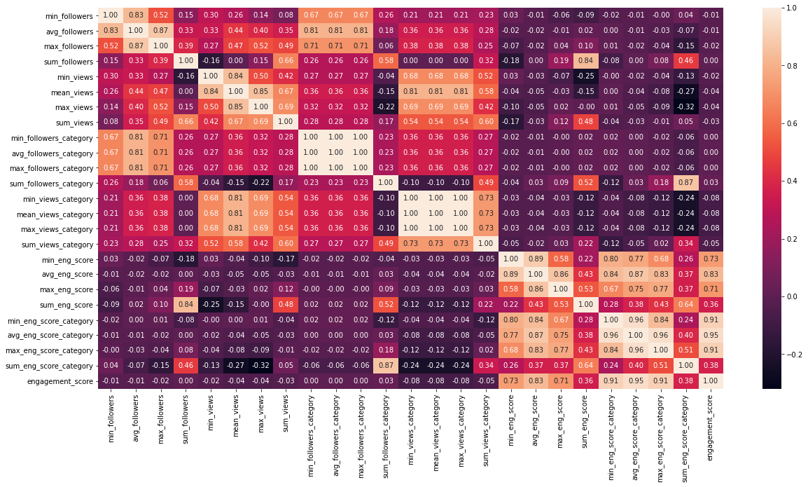
Now, let’s observe the correlation of new features. We will not include the old features since we already saw that there was no strong correlation with the target column ‘engagement_score’.

new_features=['min_followers',
 'avg_followers', 'max_followers', 'sum_followers', 'min_views',
 'mean_views', 'max_views', 'sum_views', 'min_followers_category',
 'avg_followers_category', 'max_followers_category',
 'sum_followers_category', 'min_views_category', 'mean_views_category',
 'max_views_category', 'sum_views_category', 'min_eng_score',
 'avg_eng_score', 'max_eng_score', 'sum_eng_score',
 'min_eng_score_category', 'avg_eng_score_category',
 'max_eng_score_category', 'sum_eng_score_category','engagement_score']
plt.figure(figsize=(20,10))
sns.heatmap(df_train[new_features].corr(),fmt='.2f',annot=True);

Source: Author

We have a high number of features correlation table is not clearly visible but we can still see the colour and by the colour, we can see the newly engineered features are highly correlated with target ‘engagement_score’.

Let’s just focus on the correlation with engagement_score only.

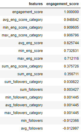
df_corr=(df_train[new_features].corr()['engagement_score']).reset_index()
df_corr.columns=['features','engagement_score']
df_corr.sort_values('engagement_score',ascending=False)

Source: Author

I have plotted the score in descending order and we can see that new features that we have created using engagement_score are highly correlated to it. Features that we have created using ‘views’ and ‘followers’ do not show much correlation to the ‘engagement_score’.

Let’s handle the Categorical features now.

Label Encoding 'gender'
gender_dict={'Male':0,'Female':1}
df_train['gender']=df_train['gender'].map(gender_dict)
df_test['gender']=df_test['gender'].map(gender_dict)

Label Encoding ‘profession’

profession_dict={'Student':0,'Working Professional':1,'Other':2}
df_train['profession']=df_train['profession'].map(profession_dict)
df_test['profession']=df_test['profession'].map(profession_dict)

Let’s try building the models now.

Model Building

We will be building ‘LinearRegression’, ‘XGBoostRegressor’, ‘RandomForestRegressor’ and ‘CatBoostRegressor’ models to solve this problem.

First, let’s select the features that we will be using.

features_to_use=['user_id', 'category_id', 'video_id', 'age', 'gender', 'profession',
 'followers', 'views', 'min_followers',
 'avg_followers', 'max_followers', 'sum_followers', 'min_views',
 'mean_views', 'max_views', 'sum_views', 'min_followers_category',
 'avg_followers_category', 'max_followers_category',
 'sum_followers_category', 'min_views_category', 'mean_views_category',
 'max_views_category', 'sum_views_category', 'min_eng_score',
 'avg_eng_score', 'max_eng_score', 'sum_eng_score',
 'min_eng_score_category', 'avg_eng_score_category',
 'max_eng_score_category', 'sum_eng_score_category']
target=['engagement_score']

While splitting the dataset into train and test it is possible that few users do not end up in the test set. Because of this when we did feature engineering and build the new features using ‘user_id’ it may be possible that test_set contains ‘NULL’ values. So we are dropping those rows.

df_test.dropna(inplace=True)

Defining X_train, y_train, X_test and y_test.

X_train,y_train=df_train[features_to_use],df_train[target]
X_test,y_test=df_test[features_to_use],df_test[target]

We will use R2_Score and Root Mean Square Value (RMSE) as performance metrics to measure the performance of the models.

def model_performance(y_test,y_pred):
 r2=round(r2_score(y_test,y_pred),3)
 rmse=round(np.sqrt(mean_squared_error(y_test,y_pred)),3)
 return r2,rmse

Building Models

model_name=['LinearRegression','XGBRegressor','RandomForestRegressor','CatBoostRegressor']
model_object=[LinearRegression(),XGBRegressor(),RandomForestRegressor(),CatBoostRegressor()]
model_r2_result=[]
model_rmse_result=[]
for i,model in enumerate(model_object):
 print('Running ',model_name[i])
 if model_name[i]=='CatBoostRegressor':
 model.fit(X_train,y_train,cat_features=['user_id', 'category_id', 'gender', 'profession'],verbose=0)
 else:
 model.fit(X_train,y_train)
 y_pred=model.predict(X_test)
 y_pred=np.array(y_pred).reshape(-1,1)
 #engagement score liest between 0 and 5. While prediting it is possible that predicted scores are beyond these
 #limits so keeping this in mind I am limiting the predictions in 0 to 5 range.
 accurate_y_pred=limit_predictions(y_pred,0,5)
 model_r2,model_rmse=model_performance(y_test,accurate_y_pred)
 model_r2_result.append(model_r2)
 model_rmse_result.append(model_rmse)

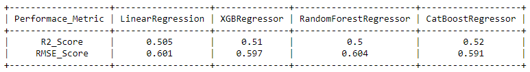
Now let’s see how the models have performed.

Model Performace

Source: Author

We can see that almost all the models have performed well on the data. CatboostRegressor got the highest R2 score and XGBRegressor got the highest RMSE_Score.

Code

Here I am presenting the complete code to solve the problem.

#importing Libraries
import pandas as pd
from catboost import CatBoostRegressor
from sklearn.linear_model import LinearRegression
from xgboost import XGBRegressor
from sklearn.ensemble import RandomForestRegressor
from sklearn.model_selection import train_test_split
import matplotlib.pyplot as plt
import seaborn as sns
from sklearn.metrics import r2_score,mean_squared_error
import numpy as np
from prettytable import PrettyTable

#Loading Data

df=pd.read_csv('train_0OECtn8.csv')

df.drop('row_id',axis=1,inplace=True)

#EDA

num_features=['age','followers','views']

cat_features=['user_id','category_id','video_id','gender','profession']

df[num_features].hist(figsize=(10,10));

sns.catplot(data=df[cat_features],kind='count',x='profession');

sns.catplot(data=df[cat_features],kind='count',x='gender');

##correlation

plt.figure(figsize=(20,10))

sns.heatmap(df.corr(),fmt='g',annot=True)

##pair plots

sns.pairplot(df)

#Feature Engineering

features=['user_id', 'category_id', 'video_id', 'age', 'gender', 'profession',

'followers', 'views']

target=['engagement_score']

x_train,x_test,y_train,y_test=train_test_split(df[features],df[target],test_size=0.2,random_state=42)

df_train=pd.concat([x_train,y_train],axis=1)

df_test=pd.concat([x_test,y_test],axis=1)

##feautures using views and followers

grp_by=['user_id']

user_id_features=df_train.groupby(grp_by)['followers'].min().reset_index()

user_id_features.rename(columns={'followers':'min_followers'},inplace=True)

user_id_features['avg_followers']=df_train.groupby(grp_by)['followers'].mean().reset_index()['followers']

user_id_features['max_followers']=df_train.groupby(grp_by)['followers'].max().reset_index()['followers']

user_id_features['sum_followers']=df_train.groupby(grp_by)['followers'].sum().reset_index()['followers']

user_id_features['min_views']=df_train.groupby(grp_by)['views'].min().reset_index()['views']

user_id_features['mean_views']=df_train.groupby(grp_by)['views'].mean().reset_index()['views']

user_id_features['max_views']=df_train.groupby(grp_by)['views'].max().reset_index()['views']

user_id_features['sum_views']=df_train.groupby(grp_by)['views'].sum().reset_index()['views']

grp_by1=['user_id','category_id']

user_id_features1=df_train.groupby(grp_by1)['followers'].min().reset_index()

user_id_features1.rename(columns={'followers':'min_followers_category'},inplace=True)

user_id_features1['avg_followers_category']=df_train.groupby(grp_by1)['followers'].mean().reset_index()['followers']

user_id_features1['max_followers_category']=df_train.groupby(grp_by1)['followers'].max().reset_index()['followers']

user_id_features1['sum_followers_category']=df_train.groupby(grp_by1)['followers'].sum().reset_index()['followers']

user_id_features1['min_views_category']=df_train.groupby(grp_by1)['views'].min().reset_index()['views']

user_id_features1['mean_views_category']=df_train.groupby(grp_by1)['views'].mean().reset_index()['views']

user_id_features1['max_views_category']=df_train.groupby(grp_by1)['views'].max().reset_index()['views']

user_id_features1['sum_views_category']=df_train.groupby(grp_by1)['views'].sum().reset_index()['views']

df_train=pd.merge(df_train,user_id_features,how='left',on=grp_by)

df_test=pd.merge(df_test,user_id_features,how='left',on=grp_by)

df_train=pd.merge(df_train,user_id_features1,how='left',on=grp_by1)

df_test=pd.merge(df_test,user_id_features1,how='left',on=grp_by1)

##features using engagement_score

grp_by=['user_id']

user_id_features2=df_train.groupby(grp_by)['engagement_score'].min().reset_index()

user_id_features2.rename(columns={'engagement_score':'min_eng_score'},inplace=True)

user_id_features2['avg_eng_score']=df_train.groupby(grp_by)['engagement_score'].mean().reset_index()['engagement_score']

user_id_features2['max_eng_score']=df_train.groupby(grp_by)['engagement_score'].max().reset_index()['engagement_score']

user_id_features2['sum_eng_score']=df_train.groupby(grp_by)['engagement_score'].sum().reset_index()['engagement_score']

grp_by1=['user_id','category_id']

user_id_features3=df_train.groupby(grp_by1)['engagement_score'].min().reset_index()

user_id_features3.rename(columns={'engagement_score':'min_eng_score_category'},inplace=True)

user_id_features3['avg_eng_score_category']=df_train.groupby(grp_by1)['engagement_score'].mean().reset_index()['engagement_score']

user_id_features3['max_eng_score_category']=df_train.groupby(grp_by1)['engagement_score'].max().reset_index()['engagement_score']

user_id_features3['sum_eng_score_category']=df_train.groupby(grp_by1)['engagement_score'].sum().reset_index()['engagement_score']

df_train=pd.merge(df_train,user_id_features2,how='left',on=grp_by)

df_test=pd.merge(df_test,user_id_features2,how='left',on=grp_by)

df_train=pd.merge(df_train,user_id_features3,how='left',on=grp_by1)

df_test=pd.merge(df_test,user_id_features3,how='left',on=grp_by1)

##correlation using new features

new_features=['min_followers',

'avg_followers', 'max_followers', 'sum_followers', 'min_views',

'mean_views', 'max_views', 'sum_views', 'min_followers_category',

'avg_followers_category', 'max_followers_category',

'sum_followers_category', 'min_views_category', 'mean_views_category',

'max_views_category', 'sum_views_category', 'min_eng_score',

'avg_eng_score', 'max_eng_score', 'sum_eng_score',

'min_eng_score_category', 'avg_eng_score_category',

'max_eng_score_category', 'sum_eng_score_category','engagement_score']

plt.figure(figsize=(20,10))

sns.heatmap(df_train[new_features].corr(),fmt='.2f',annot=True,);

##correlation only with 'engagement_score'

df_corr=(df_train[new_features].corr()['engagement_score']).reset_index()

df_corr.columns=['features','engagement_score']

df_corr.sort_values('engagement_score',ascending=False)

##Handling Categorical Data

gender_dict={'Male':0,'Female':1}

df_train['gender']=df_train['gender'].map(gender_dict)

df_test['gender']=df_test['gender'].map(gender_dict)

profession_dict={'Student':0,'Working Professional':1,'Other':2}

df_train['profession']=df_train['profession'].map(profession_dict)

df_test['profession']=df_test['profession'].map(profession_dict)

#Model Building

features_to_use=['user_id', 'category_id', 'video_id', 'age', 'gender', 'profession',

'followers', 'views', 'min_followers',

'avg_followers', 'max_followers', 'sum_followers', 'min_views',

'mean_views', 'max_views', 'sum_views', 'min_followers_category',

'avg_followers_category', 'max_followers_category',

'sum_followers_category', 'min_views_category', 'mean_views_category',

'max_views_category', 'sum_views_category', 'min_eng_score',

'avg_eng_score', 'max_eng_score', 'sum_eng_score',

'min_eng_score_category', 'avg_eng_score_category',

'max_eng_score_category', 'sum_eng_score_category']

target=['engagement_score']

#since we have a user in the data. It is possible that after splitting the dataset few users do not end up

#in test data after feature engineering. So for simplicity we are dropping null values from test data.

df_test.dropna(inplace=True)

X_train,y_train=df_train[features_to_use],df_train[target]

X_test,y_test=df_test[features_to_use],df_test[target]

def model_performance(y_test,y_pred):

r2=round(r2_score(y_test,y_pred),3)

rmse=round(np.sqrt(mean_squared_error(y_test,y_pred)),3)

return r2,rmse

def limit_predictions(y_pred,min_limit,max_limit):

new_y_pred=[]

for val in y_pred:

val=val[0] #fetching value from array

if val<=min_limit:

val=min_limit

elif val>=max_limit:

val=max_limit

new_y_pred.append(val)

return new_y_pred

Conclusion

In this article, we solved the problem of predicting how engaging a video can be at the user level.

Dataset used was from a ‘Job-a-thon’ contest organized in analytics vidya and was only available to members who have participated in the contest.

We saw that CatboostRegressor got the highest R2_Score and XGBoost got the highest RMSE_score on the data.

Read more blogs on our website.

The media shown in this article is not owned by Analytics Vidhya and are used at the Author’s discretion.

Login to continue reading and enjoy expert-curated content.

Free Courses