Bank Customer Churn Prediction Using Machine Learning

This article was published as a part of the Data Science Blogathon.

Introduction

Customer Churn prediction means knowing which customers are likely to leave or unsubscribe from your service. For many companies, this is an important prediction. This is because acquiring new customers often costs more than retaining existing ones. Once you’ve identified customers at risk of churn, you need to know exactly what marketing efforts you should make with each customer to maximize their likelihood of staying.

Customers have different behaviors and preferences, and reasons for cancelling their subscriptions. Therefore, it is important to actively communicate with each of them to keep them on your customer list. You need to know which marketing activities are most effective for individual customers and when they are most effective.

Impact of customer churn on businesses

A company with a high churn rate loses many subscribers, resulting in lower growth rates and a greater impact on sales and profits. Companies with low churn rates can retain customers.

Why is Analyzing Customer Churn Prediction Important?

Increase profits

Businesses sell products and services to make money. Therefore, the ultimate goal of churn analysis is to reduce churn and increase profits. As more customers stay longer, revenue should increase, and profits should follow.

Improve the customer experience

How does Customer Churn Prediction Work?

We first have to do some Exploratory Data Analysis in the Dataset, then fit the dataset into Machine Learning Classification Algorithm and choose the best Algorithm for the Bank Customer Churn Dataset.

Algorithms for Churn Prediction Models

XGBOOST

XGBoost, short for Extreme Gradient Boosting, is a scalable machine learning library with Distributed Gradient Boosted Decision Trees (GBDT). It provides Parallel Tree Boosting and is the leading machine learning library for regression, classification and ranking problems. To understand XGBoost, it’s important first to understand the machine learning concepts and algorithms that XGBoost is built on: supervised machine learning, decision trees, ensemble learning, and gradient boosting. Supervised machine learning uses an algorithm to train a model to find patterns in a dataset containing labels and features and then uses the trained model to predict the labels of the features in a new dataset.

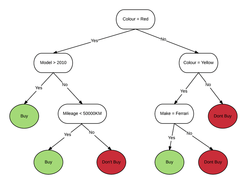
Decision trees are models that predict labels by evaluating a tree of if-then-else true/false functional questions and estimating the minimum number of questions needed to evaluate the likelihood of a correct decision. Decision trees can be used for classification to predict categories and regression to predict continuous numbers. The following simple example uses a decision tree to estimate a house’s price (tag) based on the size and number of bedrooms (features).

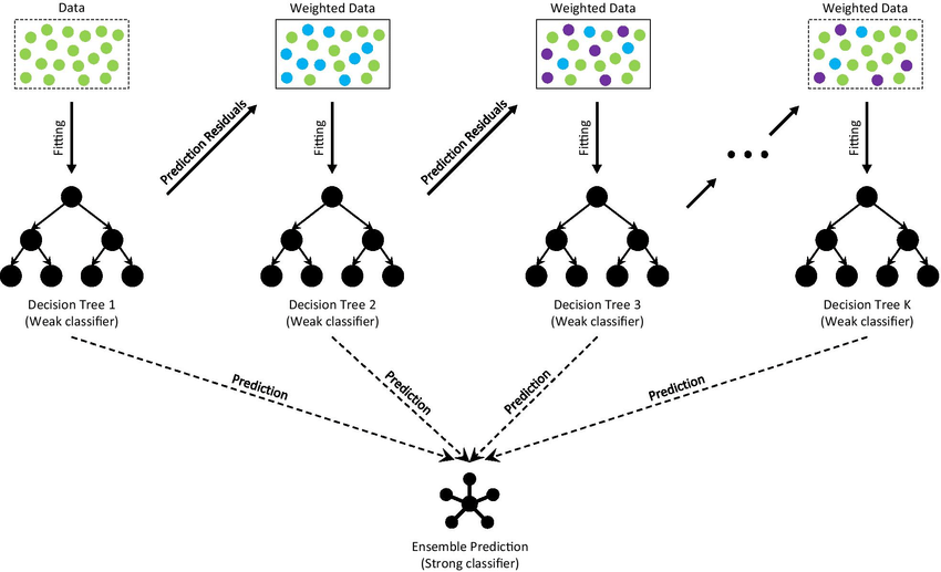
Gradient Boosted Decision Trees (GBDT) is a random forest-like decision tree ensemble learning algorithm for classification and regression. Ensemble learning algorithms combine multiple machine learning algorithms to get a better model. Both Random Forest and GBDT create models that consist of multiple decision trees. The difference is in how the trees are constructed and combined.

Decision Tree

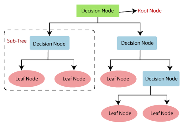
Decision trees are a nonparametric supervised learning method used for classification and regression. The goal is to build a model that predicts the value of a target variable by learning simple decision rules derived from the properties of the data. A tree can be viewed as a piecewise constant approximation.

For example, in the following example, a decision tree learns from data to approximate a sine wave using a series of if-then-else decision rules. The deeper the tree, the more complex the decision rules and the better the model.

The advantages of decision trees are:

• Easy to understand and easy to interpret. You can visualize trees.
• Little or no data preparation is required. Other techniques often require normalizing the data, creating dummy variables, and removing empty values. However, please note that this module does not support missing values.
• The cost of using a tree (predicting data) is the logarithm of the number of data points used to train the tree.
• It can handle both numeric and categorical data. However, scikit-learn’s implementation does not currently support categorical variables. Other techniques tend to specialize in analyzing datasets containing only one variable type. See Algorithms for details. Can handle multi-output issues.
• Adopted the white box model. If a given situation is observable in the model, the description of that state can be easily explained by Boolean logic. In contrast, results from black-box models (such as artificial neural networks) can be more difficult to interpret.
• Possibility to validate the model with statistical tests. This can explain the reliability of the model.
• It works well even when the assumptions are somewhat violated by the true model from which the data were generated.

The disadvantages of decision trees include:

• Decision tree learners can create overly complex trees that fail to generalize the data well. This is called overfitting. Mechanisms such as pruning, setting a minimum number of samples required at a leaf node, or setting a maximum tree depth are required to avoid this problem.
• Decision trees can be unstable. This is because small deviations in the data can produce completely different trees. This problem is mitigated by using decision trees within the ensemble. The figure above shows that the decision tree prediction is neither smooth nor continuous but a piecewise constant approximation. Therefore, they are bad at extrapolation.
• The problem of learning optimal decision trees is known to be NP-complete under some aspects of optimality and even for simple concepts. Therefore, practical decision tree learning algorithms are based on heuristic algorithms, such as the greedy algorithm, where the locally optimal decision is made at each node. Such algorithms cannot guarantee to return of globally optimal decision trees. This can be mitigated by training multiple trees in an ensemble learner and using surrogates to randomly sample features and samples.
• Some concepts, such as XOR, parity, and multiplexer problems, are difficult to master because they cannot be easily represented in decision trees.
• Decision tree learners create skewed trees when some classes are dominant. Therefore, it is recommended to balance the data set before fitting the decision tree.

Random Forest

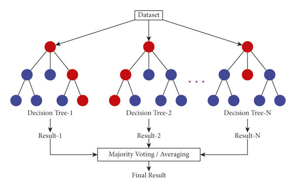
Random forest is a machine learning technique to solve regression and classification problems. It uses ensemble learning, a technique that combines many classifiers to provide solutions to complex problems.

A random forest algorithm consists of many decision trees. The “forest” created by the random forest algorithm is trained by bagging or bootstrap aggregation. Bagging is an ensemble meta-algorithm that improves the accuracy of machine learning algorithms. A (random forest) algorithm determines an outcome based on the predictions of a decision tree. Predict by averaging outputs from different trees. Increasing the number of trees improves the accuracy of the results.

Random forest removes the limitations of decision tree algorithms. Reduce data set overfitting and increase accuracy. Generate predictions without requiring a lot of configuration in your package

Support Vector Machines

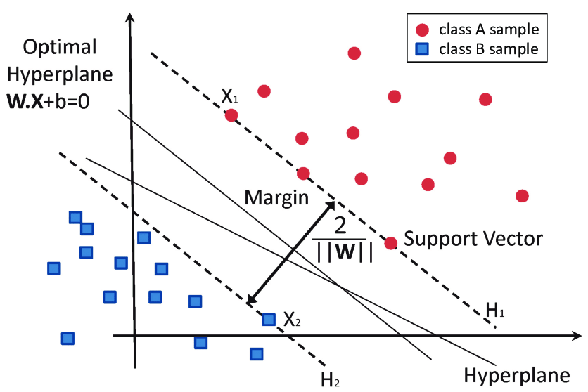
Support vector machines (SVMs) are supervised machine learning algorithms that can be used for both classification and regression tasks. However, it is mainly used in classification problems. The SVM algorithm plots each data item as a point in n-dimensional space (where n is the number of features it possesses). where the value of each feature is the value of a specific coordinate. Classification is then done by finding the hyperplane that distinguishes the two classes very well.

The advantages of support vector machines are:

• Effective in high-dimensional space.
• It works even if the number of dimensions exceeds the number of samples.
• It is also memory efficient because it uses a subset of the training points in the decision function (called support vectors).
• Versatility: You can specify different kernel functions for the decision function. A generic kernel is provided, but it is possible to specify a custom kernel.

The disadvantages of support vector machines include:

• When the number of features is much larger than the number of samples, avoiding overfitting when choosing a kernel function, the regularization term becomes important.
• SVM does not provide direct probability estimates. These are computed using an expensive 5-fold cross-validation.

Coding to Predict Bank Customer Churn Prediction

The first thing we have to do is import some libraries and datasets. You can get the dataset from here: https://www.kaggle.com/datasets/gauravtopre/bank-customer-churn-dataset

Now we have to import some libraries :

import pandas as pd
import seaborn as sns
import matplotlib.pyplot as plt
import numpy as np
sns.set_theme(color_codes=True)

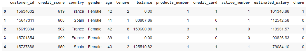
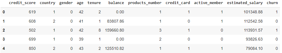
df = pd.read_csv('Bank Customer Churn Prediction.csv')
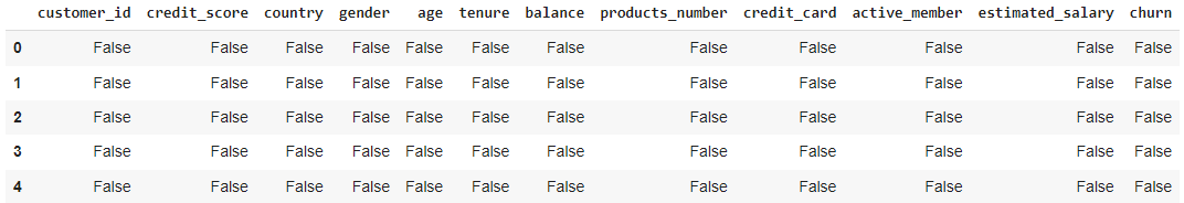
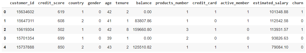
print(df.head())

Exploratory Data Analysis

The first thing we have to do in Exploratory Data Analysis is checked if there are null values in the dataset.

df.isnull().head()

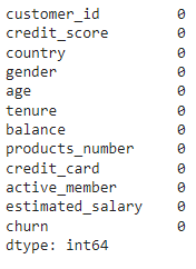
df.isnull().sum()

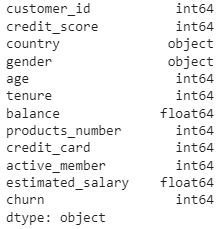
#Checking Data types
df.dtypes

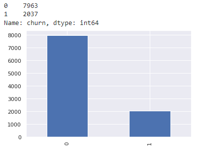
#Counting 1 and 0 Value in Churn column
color_wheel = {1: "#0392cf", 2: "#7bc043"}
colors = df["churn"].map(lambda x: color_wheel.get(x + 1))
print(df.churn.value_counts())
p=df.churn.value_counts().plot(kind="bar")

#Change value in country column
df['country'] = df['country'].replace(['Germany'],'0')
df['country'] = df['country'].replace(['France'],'1')
df['country'] = df['country'].replace(['Spain'],'2')
#Change value in gender column
df['gender'] = df['gender'].replace(['Female'],'0')
df['gender'] = df['gender'].replace(['Male'],'1')

df.head()

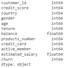
#convert object data types column to integer
df['country'] = pd.to_numeric(df['country'])
df['gender'] = pd.to_numeric(df['gender'])
df.dtypes

#Remove customer_id column
df2 = df.drop('customer_id', axis=1)
df2.head()

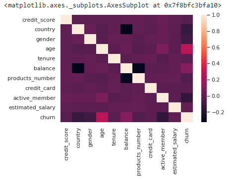
sns.heatmap(df2.corr(), fmt='.2g')

Build Machine Learning Model

X = df2.drop('churn', axis=1)
y = df2['churn']

#test size 20% and train size 80%
from sklearn.model_selection import train_test_split, cross_val_score, cross_val_predict
from sklearn.metrics import accuracy_score
X_train, X_test, y_train, y_test = train_test_split(X,y, test_size=0.2,random_state=7)

Decision Tree

from sklearn.tree import DecisionTreeClassifier
dtree = DecisionTreeClassifier()
dtree.fit(X_train, y_train)

y_pred = dtree.predict(X_test)
print("Accuracy Score :", accuracy_score(y_test, y_pred)*100, "%")

Random Forest

from sklearn.ensemble import RandomForestClassifier
rfc = RandomForestClassifier()
rfc.fit(X_train, y_train)

y_pred = rfc.predict(X_test)
print("Accuracy Score :", accuracy_score(y_test, y_pred)*100, "%")

Support Vector Machine

from sklearn import svm
svm = svm.SVC()
svm.fit(X_train, y_train)

y_pred = svm.predict(X_test)
print("Accuracy Score :", accuracy_score(y_test, y_pred)*100, "%")

XGBoost

from xgboost import XGBClassifier
xgb_model = XGBClassifier()
xgb_model.fit(X_train, y_train)

y_pred = xgb_model.predict(X_test)
print("Accuracy Score :", accuracy_score(y_test, y_pred)*100, "%")

Visualize Random Forest and XGBoost Algorithm because Random Forest and XGBoost Algorithm have the Best Accuracy

#importing classification report and confusion matrix from sklearn

from sklearn.metrics import classification_report, confusion_matrix

Random Forest

y_pred = rfc.predict(X_test)
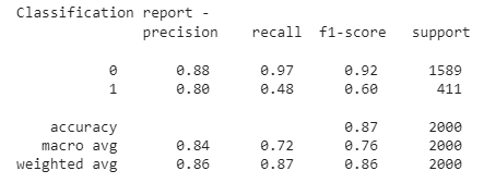
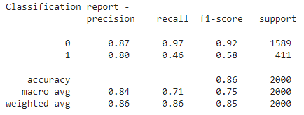
print("Classification report - n", classification_report(y_test,y_pred))

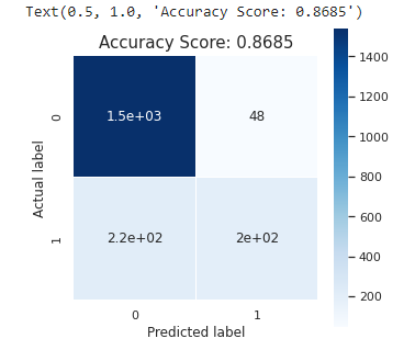
cm = confusion_matrix(y_test, y_pred)
plt.figure(figsize=(5,5))
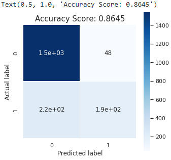
sns.heatmap(data=cm,linewidths=.5, annot=True,square = True, cmap = 'Blues')
plt.ylabel('Actual label')
plt.xlabel('Predicted label')
all_sample_title = 'Accuracy Score: {0}'.format(rfc.score(X_test, y_test))
plt.title(all_sample_title, size = 15)

from sklearn.metrics import roc_curve, roc_auc_score
y_pred_proba = rfc.predict_proba(X_test)[:][:,1]
df_actual_predicted = pd.concat([pd.DataFrame(np.array(y_test), columns=['y_actual']), pd.DataFrame(y_pred_proba, columns=['y_pred_proba'])], axis=1)
df_actual_predicted.index = y_test.index
fpr, tpr, tr = roc_curve(df_actual_predicted['y_actual'], df_actual_predicted['y_pred_proba'])
auc = roc_auc_score(df_actual_predicted['y_actual'], df_actual_predicted['y_pred_proba'])
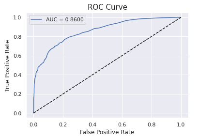
plt.plot(fpr, tpr, label='AUC = %0.4f' %auc)
plt.plot(fpr, fpr, linestyle = '--', color='k')
plt.xlabel('False Positive Rate')
plt.ylabel('True Positive Rate')
plt.title('ROC Curve', size = 15)
plt.legend()

XGBoost

y_pred = xgb_model.predict(X_test)
print("Classification report - n", classification_report(y_test,y_pred))

cm = confusion_matrix(y_test, y_pred)
plt.figure(figsize=(5,5))
sns.heatmap(data=cm,linewidths=.5, annot=True,square = True, cmap = 'Blues')
plt.ylabel('Actual label')
plt.xlabel('Predicted label')
all_sample_title = 'Accuracy Score: {0}'.format(xgb_model.score(X_test, y_test))
plt.title(all_sample_title, size = 15)

from sklearn.metrics import roc_curve, roc_auc_score
y_pred_proba = xgb_model.predict_proba(X_test)[:][:,1]
df_actual_predicted = pd.concat([pd.DataFrame(np.array(y_test), columns=['y_actual']), pd.DataFrame(y_pred_proba, columns=['y_pred_proba'])], axis=1)
df_actual_predicted.index = y_test.index
fpr, tpr, tr = roc_curve(df_actual_predicted['y_actual'], df_actual_predicted['y_pred_proba'])
auc = roc_auc_score(df_actual_predicted['y_actual'], df_actual_predicted['y_pred_proba'])
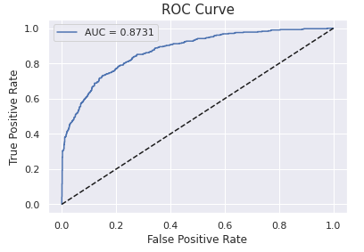
plt.plot(fpr, tpr, label='AUC = %0.4f' %auc)
plt.plot(fpr, fpr, linestyle = '--', color='k')
plt.xlabel('False Positive Rate')
plt.ylabel('True Positive Rate')
plt.title('ROC Curve', size = 15)
plt.legend()

Conclusion

The churn variable has imbalanced data. So, the solution to handle imbalanced data are :

• Resample Training set
• Use K-fold Cross-Validation in the Right Way
• Ensemble Different Resampled Datasets

We have to change the value in the Country and Gender columns so the Machine Learning model can read and predict the dataset; after changing the value, we have to change the data types on the Country and Gender column from string to integer because XGBoost Machine Learning Model cannot read string data types even though the value in the column is number.

Lastly, XGBoost and Random Forest are the best algorithms to predict Bank Customer Churn since they have the highest accuracy (86,85% and 86.45%). Random Forest and XGBoost have perfect AUC Scores. They have 0.8731 and 0.8600 AUC Scores.

I hope you liked my article on customer churn prediction. Share your views in the comments below. Read Customer Churn Prediction using MLlib here.

The media shown in this article is not owned by Analytics Vidhya and is used at the Author’s discretion.

Login to continue reading and enjoy expert-curated content.

Free Courses