Aggregating Time Series in R

Time series data can consist of the observations recorded at the specific time intervals. It can be widely used in fields such as economics, finance, environmental science, and many others. Aggregating time series data can involve summarizing the data over the specified period to extract meaningful insights. This process can be crucial when dealing with large datasets and allows for trend analysis, seasonal pattern identification, and better visualization. In this article, we will guide the concept of time series aggregation, methods to perform it, and how to implement it in the R.

Understanding Time Series Aggregation

Time series aggregation is the process of summarizing a series of data points over time. It can involve operations such as computing the mean, sum, median, or other statistical measures over the defined period (eg.., hourly, daily, weekly, monthly, etc.). Aggregation can help in reducing the noise in data, making trends more apparent and allowing for more manageable data sizes for the analysis.

It can be several reasons to aggregate the time series data:

• Smoothing Data: Aggregation can reduces the fluctuations in the data, making the trends more visible.
• Data Reduction: Summarizing the data over larger time intervals reduces the number of the observations which can be helpful when dealing with the large datasets.
• Trend Analysis: Aggregated data can allows for the easier identification of the long-term trends.

Methods of Aggregation

There are various of the method to aggregate time series data, depending on the nature of the data and the analysis objectives:

• Mean Aggregation: This method calculates the average of the data points within the each time interval.
• Sum Aggregation: This method sums all the data points within the each time interval and useful for the cumulative measures.
• Median Aggregation: This method finds the middle value of the data points within the each interval, which is less sensitive to the outliers.
• Max/Min Aggregation: This method finds the maximum or minimum value within the each time interval, useful for the range-based analysis.
• Custom Aggregation: We can also define the custom functions for the aggregation such as computing the standard deviation, variance or any other statistical measure.

Implementation in R

R can provides the several ways to perform the time series aggregation. The most commonly can be used packages are zoo, xts and dplyr, each offering functions tailored for the handling time series data.

• Using zoo and xts: These packages can be designed specifically for the time series data and offer the variety of the aggregation functions. This function in these packages can allows you to apply any function over the specified time interval.
• Using dplyr: While not specifically designed for the time series. dplyr can provides the powerful tools for the data manipulation, including the grouping date by time intervals and applying the aggregation functions.

Now we will discuss Step by Step implement the time series aggregation in R Programming Language.

Step 1: Install and Load Required Packages

First, we will need to install and load the necessary R packages. For this example, we will use the zoo package which can be designed for the working with time series data.

Step 2: Create the Sample Time Series Dataset

Next, we will create the sample time series dataset. Let's assume we have daily temperature the data for the entire year.

Output:

2023-01-01 2023-01-02 2023-01-03 2023-01-04 2023-01-05 2023-01-06 
 17.19762 18.84911 27.79354 20.35254 20.64644 28.57532 

Step 3: Aggregate the Time Series Data

Now, lets aggregate this daily data into the monthly and quarterly averages. It can help us to analyze the trends at the higher level, making it easier to identify patterns.

1. Aggregate By Month

To aggregate the data by month, we will use the aggregate function. We will calculate the average temperature for the each month.

Output:

Jan 2023 Feb 2023 Mar 2023 Apr 2023 May 2023 Jun 2023 Jul 2023 Aug 2023 Sep 2023 
19.84086 20.84067 20.15299 19.53056 19.23876 20.46007 20.30120 19.54078 20.63493 
Oct 2023 Nov 2023 Dec 2023 
20.66933 21.02647 19.77436 

2. Aggregate By Quarter

We can aggregate the data by the quator. It will calculate the average temperature for the each quarter.

Output:

 2023 Q1 2023 Q2 2023 Q3 2023 Q4 
20.25942 19.73759 20.15379 20.48423 

Step 4: Visualize the Aggregated Data

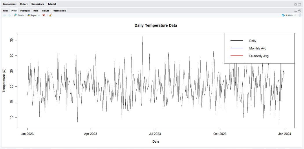
Visualizing the aggregated data can help you better understand the trends. We will plot the original daily data along with the monthly and quarterly averages.

Output:

Now that we have aggregated the data and visualized it, we can interpret the results:

• Daily Data: The black line can represents the original daily temperature data, showing the fluctuations due to the daily variations.
• Monthly aggregation: The blue line shows the average temperature for the each month. This smooth out the daily fluctuations and highlights the monthly trends.
• Quarterly Aggregation: The red line shows the average temperature for the each quarter, providing the even smoother view that highlights longer-term trends.

Conclusion

Aggregating time series data is the powerful technique that helps in the simplifying and summarizing the large datasets. Making it easier to analyze the trends, patterns and the other key insights. R can provides the verstaile tools through the packages like zoo,xts and dplyr to perform the various aggregation operations. By understanding and applying these techniques , we can enhance the time series analysis and derive more meaningful conclusions from the data.