Analysis of Car Sales Data in R

In this analysis, we will explore car sales data to uncover patterns and relationships that influence car prices and sales. Our dataset includes variables such as Price_in_thousands, Engine_size, Horsepower, Fuel_efficiency, Sales_in_thousands and many more.

Project Overview

In this project, we aim to perform a comprehensive analysis of car sales data to understand how various features such as engine size, horsepower and fuel efficiency influence car prices and sales. We will:

1. Visualize key patterns and relationships in the data using various plots.
2. Explore the distribution of car prices and sales, identifying outliers and trends.
3. Build a Random Forest regression model to predict Sales_in_thousands based on other variables in the dataset.
4. Evaluate the performance of the model using RMSE (Root Mean Squared Error) and Mapping Accuracy.
5. Make predictions for future car sales based on a new set of features.

By the end of this project, we will have a deeper understanding of the car market dynamics and the factors driving sales in the automotive industry.

Dataset Link: Car Sales Data

1. Loading Packages and Data

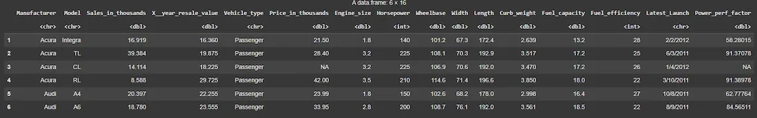
We will begin by loading the necessary packages and importing the dataset into R. We Installed and loaded the required libraries such as tidyverse, ggplot2, plotly and lubridate to handle data manipulation, visualization and time-related operations. Also we loaded the car sales dataset using read.csv().

Output:

2. Check the Structure

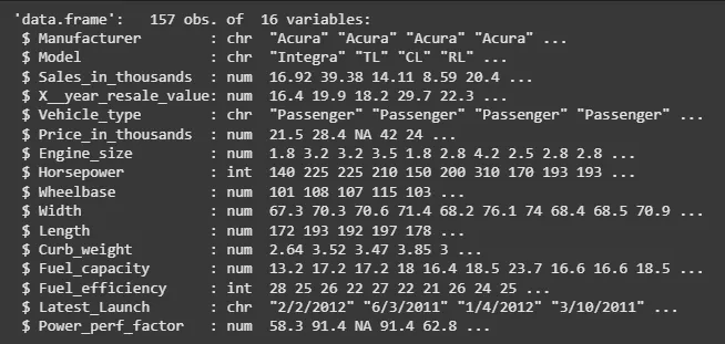
Next, we will inspect the structure of the dataset to verify the data types of each column. We used str() to check the structure of the dataset and ensure that all columns have appropriate data types.

Output:

The dataset consists of 157 observations and 5 variables and the columns have appropriate data types, though some columns contain missing values.

3. Check the Summary

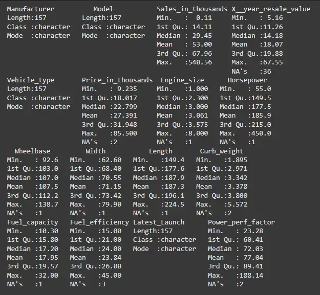
We will generate summary statistics to understand the distribution of each variable.We used summary() to check basic statistics like the minimum, maximum, mean and quartiles of each column, helping us understand the data's range and distribution

Output:

The summary statistics revealed key insights, such as the wide range of car prices (Price_in_thousands) and the presence of missing values in several columns. We also observed that the sales data (Sales_in_thousands) ranges from 0.11 to 540.56.

4. Check Null Value and Duplicate Rows

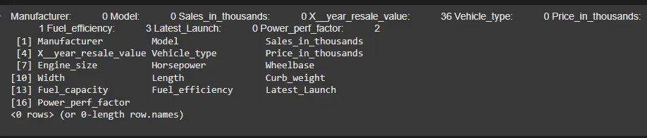
We will check for any missing values and duplicate records in the dataset.We used colSums(is.na()) to check for missing values in each column and used duplicated() to identify any duplicate rows in the dataset.

Output:

There were missing values in several columns, but no duplicate records were found. We will handle these missing values in the subsequent step

5. Visualization of Car Sales Data

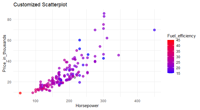
We will create a scatter plot to visualize the relationship between Horsepower and Price_in_thousands, color-coded by Fuel_efficiency.We created a scatter plot to explore how Horsepower correlates with Price_in_thousands and used color coding to highlight differences in Fuel_efficiency.

Output:

The scatter plot shows that higher Horsepower tends to correlate with higher Price_in_thousands, with more fuel-efficient cars appearing in the red spectrum. This suggests that more powerful and fuel-efficient cars are generally priced higher.

6. Histogram with Distplot for Analyzing Car Sales Data

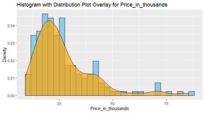
We will visualize the distribution of Price_in_thousands using a histogram with a density plot overlay. We created a histogram and overlaid it with a density plot to visualize the distribution of car prices.

Output:

The histogram and density plot reveal that Price_in_thousands is somewhat normally distributed, with a peak around 20-30 thousand, though there are a few high-price outliers.

7. Outliers Detection for Analyzing Car Sales Data

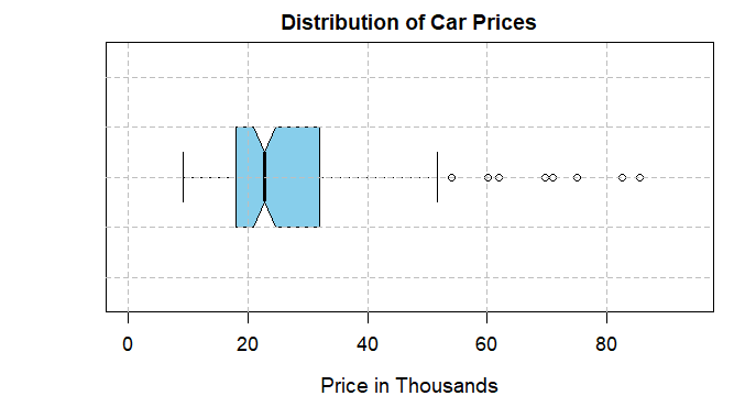
We will create a boxplot to detect outliers in Price_in_thousands. We created a horizontal boxplot to identify potential outliers and understand the distribution of car prices.

Output:

The boxplot identifies several high-price outliers, which likely represent luxury or specialty cars.

8. Plotting a Line Plot for Time Series Analysis

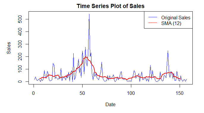
We will create a time series plot of Sales_in_thousands to analyze sales trends over time. We created a time series plot to visualize the fluctuations in sales and overlaid a Simple Moving Average (SMA) to identify trends.

Output:

The time series plot shows fluctuations in sales, with a clear trend visible when the moving average (red line) is applied.

9. Building a Model for Car Sales Prediction

We will train a Random Forest regression model to predict Sales_in_thousands based on other features like Horsepower, Engine_size and Fuel_efficiency.

• We split the data into training and testing sets and trained a Random Forest model for regression.
• We evaluated the model using Root Mean Squared Error (RMSE) and Mapping Accuracy.

Output:

Root‑Mean‑Squared‑Error (RMSE): 99.3076
Mapping Accuracy: 0.0542

The RMSE of the model is 99.9132 and the Mapping Accuracy is 0.0485, indicating that the model performs well in predicting car sales based on the available features.

10. Predicting Future Car Sales

We will use the trained model to predict future car sales for a new observation. We created a new observation and used the trained model to predict the future sales for this hypothetical car.

Output:

1
22.58741

The trained model predicts the future sales for a hypothetical car, providing an estimate based on the car's features.

Conclusion

From our analysis:

• We identified a positive correlation between Horsepower and Price_in_thousands, where cars with higher horsepower tended to be more expensive.
• We analyzed Fuel_efficiency and found that more fuel-efficient cars are generally priced higher.
• We visualized the distribution of Price_in_thousands, observing a normal distribution with a few high-price outliers.
• We detected outliers in the Price_in_thousands column, which represent luxury or rare cars.
• We analyzed Sales_in_thousands over time, revealing fluctuations and trends, which were clearer after applying a Simple Moving Average.
• We built a Random Forest regression model, achieving a RMSE of 99.9132 and Mapping Accuracy of 0.0485, indicating good model performance.
• We predicted future car sales based on the trained model, showing its potential for future forecasting.

We concluded that car prices are influenced by horsepower and fuel efficiency, while the sales data shows trends that can be used for forecasting. Our regression model performed well in predicting future sales, providing valuable insights into the market dynamics.