Bernoulli Distribution in R

In R language there are various ways to simulate, visualize, and work with Bernoulli-distributed data. This article provides a complete theoretical background, practical examples, and applications of the Bernoulli distribution in R.

Bernoulli Distribution in R

Bernoulli Distribution is a special case of Binomial distribution where only a single trial is performed. It is a discrete probability distribution for a Bernoulli trial (a trial that has only two outcomes i.e. either success or failure). For example, In R it can be represented as a coin toss where the probability of getting the head is 0.5 and getting a tail is 0.5. It is a probability distribution of a random variable that takes value 1 with probability p and the value 0 with probability q=1-p. The Bernoulli distribution is a special case of the binomial distribution with n=1.

The probability mass function f of this distribution, over possible outcomes k, is given by :

The above relation can also be expressed as:

In R Programming Language, there are 4 built-in functions to for Bernoulli distribution and all of them are discussed below.

1: dbern()

dbern( ) function in R programming measures the density function of the Bernoulli distribution.  

Syntax: dbern(x, prob, log = FALSE)

Parameter:

• x: vector of quantiles
• prob: probability of success on each trial
• log: logical; if TRUE, probabilities p are given as log(p)

In statistics, it is given by below formula:

Now we will plot Bernoulli distribution using dbern function.

Output:

2: pbern() 

pbern( ) function in R programming giver the distribution function for the Bernoulli distribution. The distribution function or cumulative distribution function (CDF) or cumulative frequency function, describes the probability that a variate X takes on a value less than or equal to a number x.

Syntax: pbern(q, prob, lower.tail = TRUE, log.p = FALSE)

Parameter:

• q: vector of quantiles
• prob: probability of success on each trial
• lowe.tail: logical
• log.p: logical; if TRUE, probabilities p are given as log(p).

Now we will plot Bernoulli distribution using pbern function.

Output:

The above plot represents the Cumulative Distribution Function of Bernoulli Distribution in R.

3: qbern()

qbern( ) gives the quantile function for the Bernoulli distribution. A quantile function in statistical terms specifies the value of the random variable such that the probability of the variable being less than or equal to that value equals the given probability.

Syntax: qbern(p, prob, lower.tail = TRUE, log.p = FALSE)

Parameter:

• p: vector of probabilities.
• prob: probability of success on each trial.
• lower.tail: logical
• log.p: logical; if TRUE, probabilities p are given as log(p).

Now we will plot Bernoulli distribution using qbern function.

Output:

4: rbern()

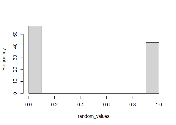
rbern( ) function in R programming is used to generate a vector of random numbers which are Bernoulli distributed.

Syntax: rbern(n, prob)

Parameter:

• n: number of observations.
• prob: number of observations.

Now we will plot Bernoulli distribution using rbern function.

Output: 

 [1] 0 0 0 1 0 1 1 0 0 1 0 1 1 1 0 0 0 0 1 0 1 0 1 0 0 0 0 1 1 0 0 0 0 1 0 0 0 0 1 0
 [41] 1 0 1 0 1 1 0 1 1 0 0 0 0 0 1 0 1 0 0 1 0 1 0 0 0 1 0 1 0 0 0 1 0 0 1 1 0 1 1 0
 [81] 1 0 0 0 1 0 0 1 1 0 1 1 0 1 1 1 1 1 0 1

The above plot represents Randomly Drawn Numbers of Bernoulli Distribution in R.

Applications of Bernoulli Distribution

Here are the some main Applications of Bernoulli Distribution.

1. The Bernoulli distribution is frequently used in machine learning and data analysis for binary classification tasks. It can simulate the likelihood that a sample will fall into a specific class or category.
2. The Bernoulli distribution is used to model click-through rates (CTR) in online advertising and marketing. The distribution can be used to calculate the likelihood that a user will click on an advertisement or perform a particular activity.
3. To ascertain if a product or procedure complies with specific criteria, the Bernoulli distribution is used in quality control. It is possible to utilize it to simulate the occurrence of flaws or failures.
4. When analyzing survey data, binary replies to questions with true/false or yes/no alternatives can be modeled using the Bernoulli distribution. This makes it possible to estimate response probabilities and compare proportions.
5. Clinical trials and epidemiological research are two examples of biological investigations that make use of the Bernoulli distribution. It can simulate things like the onset of an illness, the efficacy or inefficacy of treatments, or patient reactions.
6. In reliability engineering, binary events linked to system dependability, such as component failure or system downtime, can be analyzed using the Bernoulli distribution.
7. The Bernoulli distribution is used to represent the probability of uncommon events or insurance claims in risk assessment and insurance studies.

Conclusion

The Bernoulli distribution is a foundational concept in probability and statistics. It models binary outcomes and serves as the basis for more complex distributions like the binomial distribution. In R, working with Bernoulli trials is straightforward using functions like rbinom(), dbinom(), and pbinom(). Through simulation, visualization, and real-world applications, you can better understand how the Bernoulli distribution can be used to model random binary outcomes in various domains.