Bootstrap Confidence Interval with R Programming

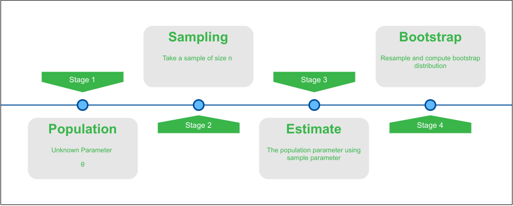
Bootstrapping is a statistical method for inference about a population using sample data. It can be used to estimate the confidence interval(CI) by drawing samples with replacement from sample data. Bootstrapping can be used to assign CI to various statistics that have no closed-form or complicated solutions. Suppose we want to obtain a 95% confidence interval using bootstrap resampling the steps are as follows: 

1. Sample n elements with replacement from original sample data.
2. For every sample calculate the desired statistic eg. mean, median etc.
3. Repeat steps 1 and 2 m times and save the calculated stats.
4. Plot the calculated stats which forms the bootstrap distribution
5. Using the bootstrap distribution of desired stat we can calculate the 95% CI

Illustration of the bootstrap distribution generation from sample: 

👁 Bootstrap generation process

Implementation in R

In R Programming the package boot allows a user to easily generate bootstrap samples of virtually any statistic that we can calculate. We can generate estimates of bias, bootstrap confidence intervals, or plots of bootstrap distribution from the calculated from the boot package.

For demonstration purposes, we are going to use the iris dataset due to its simplicity and availability as one of the built-in datasets in R. The data set consists of 50 samples from each of the three species of Iris (Iris setosa, Iris Virginia, and Iris versicolor). Four features were measured from each sample: the length and the width of the sepals and petals, in centimeters. We can view the iris dataset using head command and note the features of interests. 

Output: 

 Sepal.Length Sepal.Width Petal.Length Petal.Width Species
 5.1 3.5 1.4 0.2 setosa

We want to estimate the correlation between Petal Length and Petal Width. 

Steps to Compute the Bootstrap CI in R:

1. Import the boot library for calculation of bootstrap CI and ggplot2 for plotting. 
 

2. Create a function that computes the statistic we want to use such as mean, median, correlation, etc. 

3. Using the boot function to find the R bootstrap of the statistic. 

Output: 

ORDINARY NONPARAMETRIC BOOTSTRAP


Call:
boot(data = iris, statistic = corr.fun, R = 1000)


Bootstrap Statistics :
 original bias std. error
t1* 0.9376668 -0.002717295 0.009436212

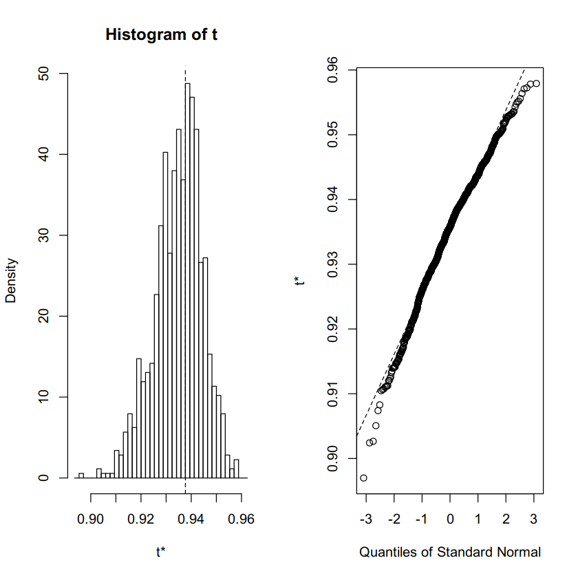
4. We can plot the generated bootstrap distribution using the plot command with calculated bootstrap. 

Output: 

👁 output-plot

5. Using the boot.ci() function to get the confidence intervals. 

Output: 

BOOTSTRAP CONFIDENCE INTERVAL CALCULATIONS
Based on 1000 bootstrap replicates

CALL : 
boot.ci(boot.out = bootstrap, type = c("norm", "basic", "perc", 
 "bca"))

Intervals : 
Level Normal Basic 
95% ( 0.9219, 0.9589 ) ( 0.9235, 0.9611 ) 

Level Percentile BCa 
95% ( 0.9142, 0.9519 ) ( 0.9178, 0.9535 ) 
Calculations and Intervals on Original Scale

Inference for Bootstrap CI From the Output:

Looking at the Normal method interval of (0.9219, 0.9589) we can be 95% certain that the actual correlation between petal length and width lies in this interval 95% of the time. As we have seen the output consists of multiple CI using different methods according to the type parameter in function boot.ci. The computed intervals correspond to the ("norm", "basic", "perc", "bca") or Normal, Basic, Percentile, and BCa which give different intervals for the same level of 95%. The specific method to use for any variable depends on various factors such as its distribution, homoscedastic, bias, etc.

The 5 methods that boot package provides for bootstrap confidence intervals are summarized below:

1. Normal bootstrap or Standard confidence limits methods use the standard deviation for calculation of CI. 
   
   • Use when statistic is unbiased.
   • Is normally distributed.
2. Basic bootstrap or Hall's (second percentile) method use percentile to calculate upper and lower limit of test statistic. 
   
   • When statistic is unbiased and homoscedastic.
   • The bootstrap statistic can be transformed to a standard normal distribution.
3. Percentile bootstrap or Quantile-based, or Approximate intervals use quantiles eg 2.5%, 5% etc. to calculate the CI. 
   
   • Use when statistic is unbiased and homoscedastic.
   • The standard error of your bootstrap statistic and sample statistics are the same.
4. BCa bootstrap or Bias Corrected Accelerated use percentile limits with bias correction and estimate acceleration coefficient corrects the limit and find the CI. 
   
   • The bootstrap statistic can be transformed to a normal distribution.
   • The normal-transformed statistic has a constant bias.
5. Studentized bootstrap resamples the bootstrap sample to find a second-stage bootstrap statistic and use it to calculate the CI. 
   
   • Use when statistic is homoscedastic.
   • The standard error of bootstrap statistic can be estimated by second-stage resampling.

References : 
R bootstrap package Boot 
Bootstrapping Statistics Wikipedia 
Bootstrap for Confidence Interval