 |
VOOZH | about |
|
VOOZH | about |
getwd() function and place out datasets binary.csv inside it to proceed further.
Output:
'data.frame': 400 obs. of 4 variables:
 $ admit: int 0 1 1 1 0 1 1 0 1 0 ...
 $ gre : int 380 660 800 640 520 760 560 400 540 700 ...
 $ gpa : num 3.61 3.67 4 3.19 2.93 3 2.98 3.08 3.39 3.92 ...
 $ rank : int 3 3 1 4 4 2 1 2 3 2 ...
Looking at the structure of the datasets we can observe that it has 4 variables, where admit tells whether a candidate will get admitted or not admitted (1 if admitted and 0 if not admitted) gre, gpa and rank give the candidates gre score, his/her gpa in the previous college and previous college rank respectively. We use admit as the dependent variable and gre, gpa, and rank as the independent variables. Now understand the whole process in a stepwise manner
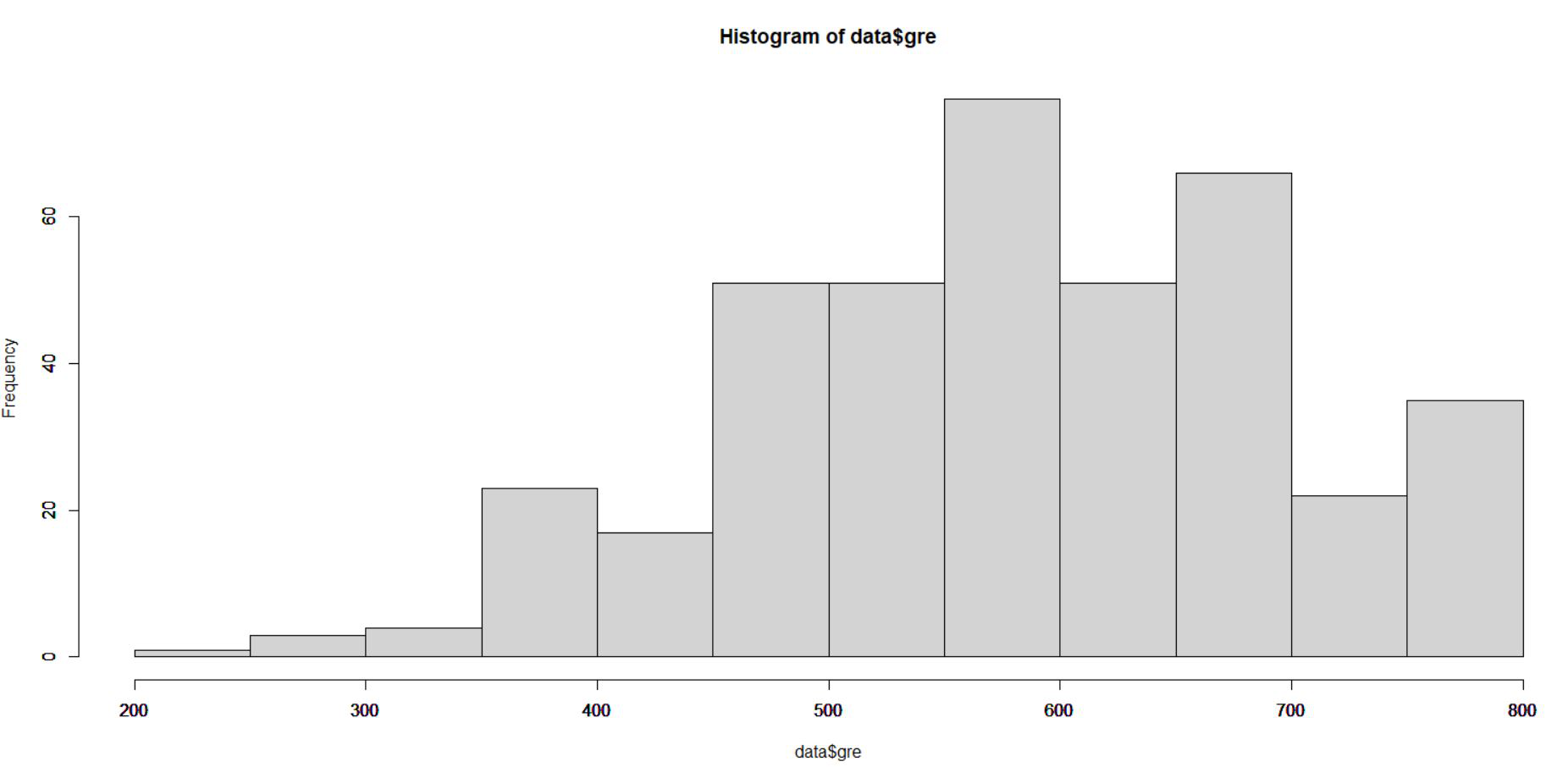
Step 1: Scaling of the data To set up a neural network to a dataset it is very important that we ensure a proper scaling of data. The scaling of data is essential because otherwise, a variable may have a large impact on the prediction variable only because of its scale. Using unscaled data may lead to meaningless results. The common techniques to scale data are min-max normalization, Z-score normalization, median and MAD, and tan-h estimators. The min-max normalization transforms the data into a common range, thus removing the scaling effect from all the variables. Here we are using min-max normalization for scaling data. Output: 👁 Unscaled Data Representationnormalize <- function(x) {
return ((x - min(x)) / (max(x) - min(x)))
}
Output:
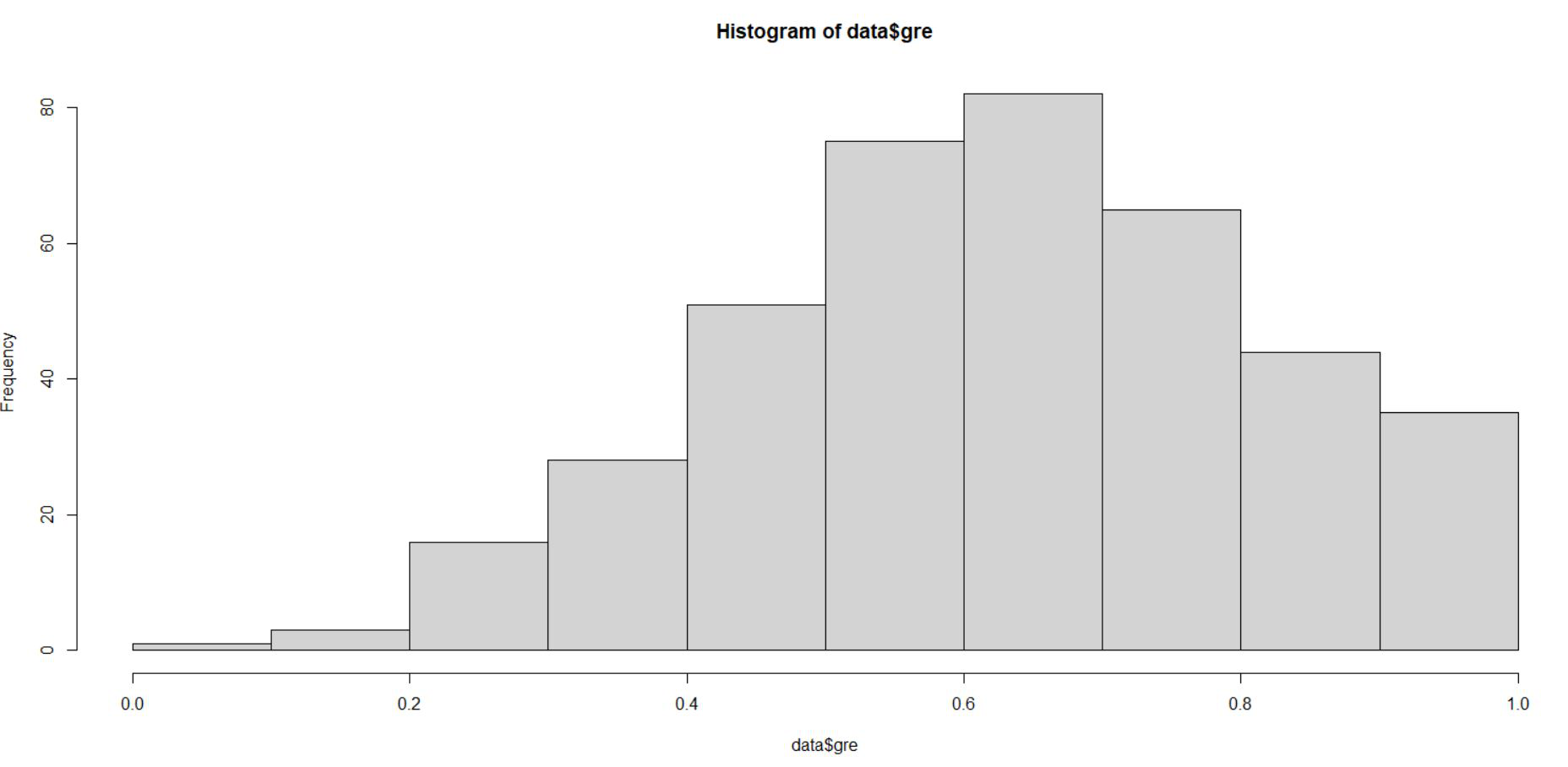
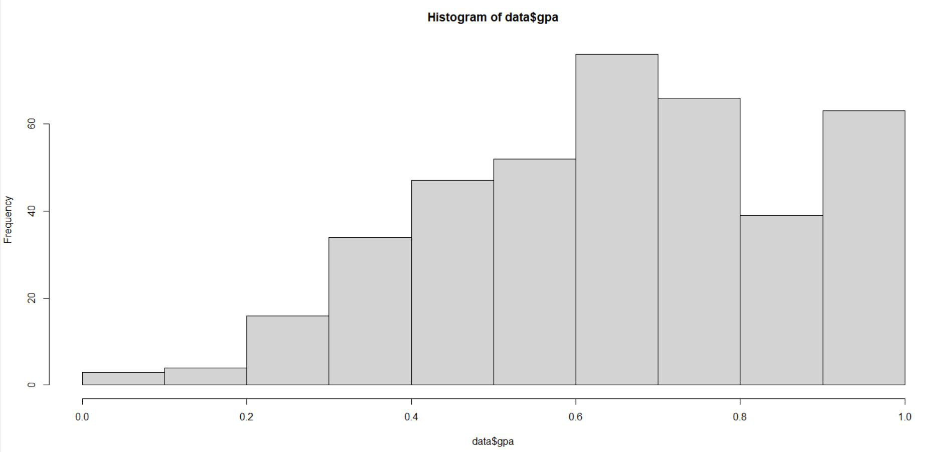
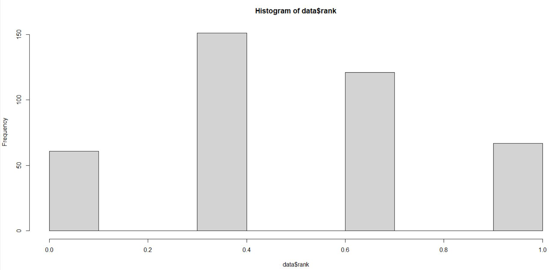
👁 Scaled data$greFrom the above representation we can see that gre data is scaled in the range of 0 to 1. Similar we do for gpa and rank.
Output: 👁 Scaled data$gpaNow divide the data into a training set and test set. The training set is used to find the relationship between dependent and independent variables while the test set analyses the performance of the model. We use 60% of the dataset as a training set. The assignment of the data to training and test set is done using random sampling. We perform random sampling on R using sample() function. Use set.seed()to generate same random sample every time and maintain consistency. Use the index variable while fitting neural network to create training and test data sets. The R script is as follows:
set.seed(222)
inp<-sample(2,nrow(data),replace=TRUE,prob=c(0.7,0.3))
training_data<-data[inp==1,]
test_data<-data[inp==2,]
Now fit a neural network on our data. We use neuralnet library for the same. neuralnet() function helps us to establish a neural network for our data. The neuralnet() function we are using here has the following syntax.
Syntax: neuralnet(formula, data, hidden = 1, stepmax = 1e+05, rep = 1, lifesign = "none", algorithm = "rprop+", err.fct = "sse", linear.output = TRUE)Parameters:
| Argument | Description |
|---|---|
| formula | a symbolic description of the model to be fitted. |
| data | a data frame containing the variables specified in formula. |
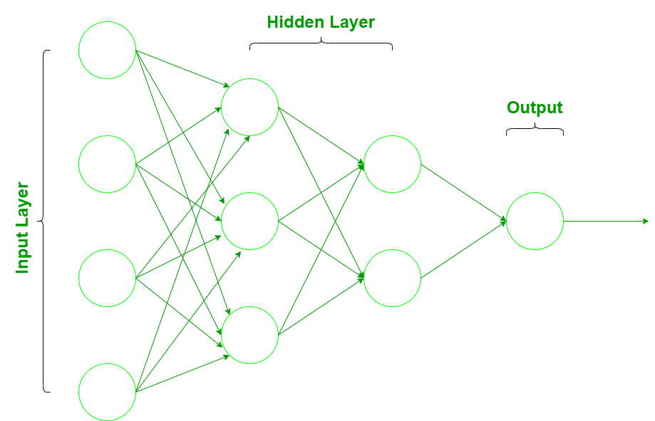
| hidden | a vector of integers specifying the number of hidden neurons (vertices) in each layer |
| err.fct | a differentiable function that is used for the calculation of the error. Alternatively, the strings ‘sse’ and ‘ce’ which stand for the sum of squared errors and the cross-entropy can be used. |
| linear.output | logical. If act.fct should not be applied to the output neurons set linear output to TRUE, otherwise to FALSE. |
| lifesign | a string specifying how much the function will print during the calculation of the neural network. ‘none’, ‘minimal’ or ‘full’. |
| rep | the number of repetitions for the neural network’s training. |
| algorithm | a string containing the algorithm type to calculate the neural network. The following types are possible: ‘backprop’, ‘rprop+’, ‘rprop-‘, ‘sag’, or ‘slr’. ‘backprop’ refers to backpropagation, ‘rprop+’ and ‘rprop-‘ refer to the resilient backpropagation with and without weight backtracking, while ‘sag’ and ‘slr’ induce the usage of the modified globally convergent algorithm (grprop). |
| stepmax | the maximum steps for the training of the neural network. Reaching this maximum leads to a stop of the neural network’s training process. |
hidden: 5 thresh: 0.01 rep: 1/2 steps: 1000 min thresh: 0.092244246452834
 2000 min thresh: 0.092244246452834
 3000 min thresh: 0.092244246452834
 4000 min thresh: 0.092244246452834
 5000 min thresh: 0.092244246452834
 6000 min thresh: 0.092244246452834
 7000 min thresh: 0.092244246452834
 8000 min thresh: 0.0657773918077728
 9000 min thresh: 0.0492128119805471
 10000 min thresh: 0.0350341801886022
 11000 min thresh: 0.0257113452845989
 12000 min thresh: 0.0175961794629306
 13000 min thresh: 0.0108791716102531
 13253 error: 139.80883 time: 7.51 secs
hidden: 5 thresh: 0.01 rep: 2/2 steps: 1000 min thresh: 0.147257381292693
 2000 min thresh: 0.147257381292693
 3000 min thresh: 0.091389043508166
 4000 min thresh: 0.0648814957085886
 5000 min thresh: 0.0472858320232246
 6000 min thresh: 0.0359632940146351
 7000 min thresh: 0.0328699898176084
 8000 min thresh: 0.0305035254157369
 9000 min thresh: 0.0305035254157369
 10000 min thresh: 0.0241743801258625
 11000 min thresh: 0.0182557959333173
 12000 min thresh: 0.0136844933371039
 13000 min thresh: 0.0120885410813301
 14000 min thresh: 0.0109156031403791
 14601 error: 147.41304 time: 8.25 secs
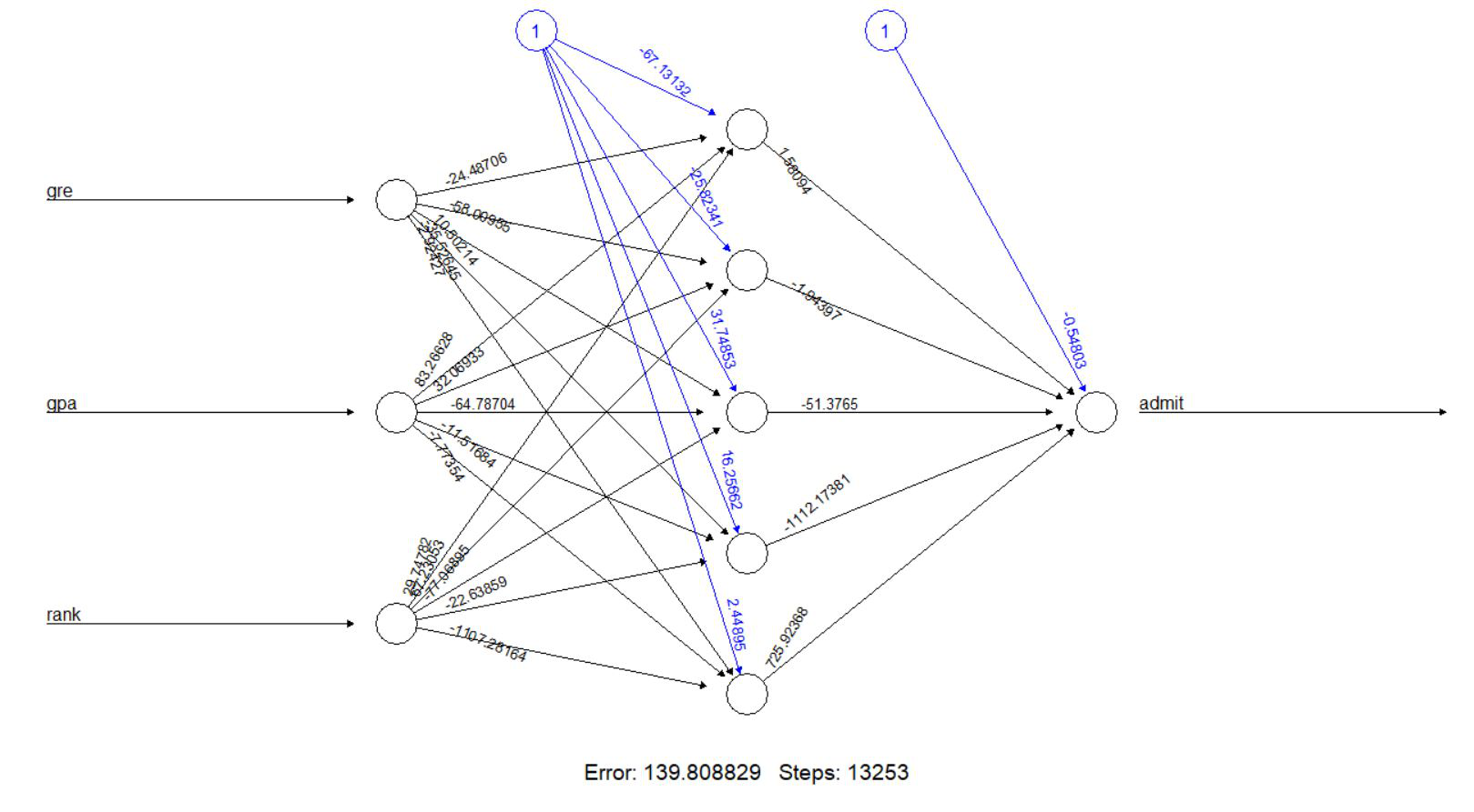
From the above output we conclude that both of the repetitions converge. But we will use the output-driven in the first repetition because it gives less error(139.80883) than the error(147.41304) the second repetition derives. Now, lets plot our neural network and visualize the computed neural network.
Output: 👁 Plot[, 1] [, 2] error 1.398088e+02 1.474130e+02 reached.threshold 9.143429e-03 9.970574e-03 steps 1.325300e+04 1.460100e+04 Intercept.to.1layhid1 -6.713132e+01 -1.136151e+02 gre.to.1layhid1 -2.448706e+01 1.469138e+02 gpa.to.1layhid1 8.326628e+01 1.290251e+02 rank.to.1layhid1 2.974782e+01 -5.733805e+01 Intercept.to.1layhid2 -2.582341e+01 2.508958e-01 gre.to.1layhid2 -5.800955e+01 1.302115e+00 gpa.to.1layhid2 3.206933e+01 -4.856419e+00 rank.to.1layhid2 6.723053e+01 1.540390e+01 Intercept.to.1layhid3 3.174853e+01 -3.495968e+01 gre.to.1layhid3 1.050214e+01 1.325498e+02 gpa.to.1layhid3 -6.478704e+01 -4.536649e+01 rank.to.1layhid3 -7.706895e+01 -1.844943e+02 Intercept.to.1layhid4 1.625662e+01 2.188646e+01 gre.to.1layhid4 -3.552645e+01 1.956271e+01 gpa.to.1layhid4 -1.151684e+01 2.052294e+01 rank.to.1layhid4 -2.263859e+01 1.347474e+01 Intercept.to.1layhid5 2.448949e+00 -3.978068e+01 gre.to.1layhid5 -2.924269e+00 -1.569897e+02 gpa.to.1layhid5 -7.773543e+00 1.500767e+02 rank.to.1layhid5 -1.107282e+03 4.045248e+02 Intercept.to.admit -5.480278e-01 -3.622384e+00 1layhid1.to.admit 1.580944e+00 1.717584e+00 1layhid2.to.admit -1.943969e+00 -6.195182e+00 1layhid3.to.admit -5.137650e+01 6.731498e+00 1layhid4.to.admit -1.112174e+03 -4.245278e+00 1layhid5.to.admit 7.259237e+02 1.156083e+01Step 4: Prediction
Let's predict the rating using the neural network model. We must remember that the predicted rating will be scaled and it must be transformed in order to make a comparison with the real rating. Also compare the predicted rating with real rating.
Output:[, 1] 2 0.34405929 3 0.41148373 4 0.07642387 7 0.98152454 8 0.26230256 9 0.07660906Output:
 admit gre gpa rank
2 1 0.7586207 0.8103448 0.6666667
Step 5: Confusion Matrix and Misclassification error
Then, we round up our results using compute() method and create a confusion matrix to compare the number of true/false positives and negatives. We will form a confusion matrix with training data
 pred1 0 1
 0 177 58
 1 12 34
The model generates 177 true negatives (0’s), 34 true positives (1’s), while there are 12 false negatives and 58 false positives. Now, lets calculate the misclassification error (for training data) which {1 - classification error}
Output:[1] 0.2491103
The misclassification error comes out to be 24.9%. We can further increase the accuracy and efficiency of our model by increasing of decreasing nodes and bias in hidden layers .
The strength of machine learning algorithms lies in their ability to learn and improve every time in predicting an output. In the context of neural networks, it implies that the weights and biases that define the connection between neurons become more precise. This is why the weights and biases are selected such as the output from the network approximates the real value for all the training inputs. Similarly, we can make more efficient neural network models in R to predict and drive decisions.