Compute Empirical Cumulative Distribution Function in R

The Empirical Cumulative Distribution Function (ECDF) is a non-parametric method for estimating the Cumulative Distribution Function (CDF) of a random variable. Unlike parametric methods, the ECDF makes no assumptions about the underlying probability distribution of the data.

It is defined as a step function that increases by at each observed data point, where is the total number of observations in the dataset.

The ECDF is a useful tool for visualizing the distribution of a dataset and can provide insights into the underlying distribution that would be difficult to obtain through traditional summary statistics.

Prerequisites

Before getting into the details of the Empirical Cumulative Distribution Function (ECDF), it’s important to understand a few foundational concepts related to probability distributions:

1. Probability Density Function (PDF)

• The probability density function (PDF) describes the probability distribution of a continuous random variable. It is defined as the derivative of the cumulative distribution function (CDF):

• Here, is the cumulative distribution function and represents the rate at which the probability accumulates with respect to .

2. Probability Mass Function (PMF)

• The probability mass function (PMF) is used for discrete random variables. It gives the probability that the variable takes a specific value:

• where is a discrete random variable and is a particular value in its range.

3. Cumulative Distribution Function (CDF)

• The cumulative distribution function (CDF) gives the probability that a random variable is less than or equal to a particular value . It is defined as:

• The CDF can be defined for both discrete and continuous variables and it is a non-decreasing function ranging from 0 to 1.

Mathematical Concept of ECDF

The ECDF is defined as follows:

• Let    be a random sample of size n from a distribution with CDF  . The ECDF is given by:

• where,

.

Mean and Variance

• The ECDF can be used to estimate the mean and variance of a distribution.
• The mean of the distribution can be estimated as the area under the curve of the ECDF:

• The variance of the distribution can be estimated as:

• The ECDF can also be used to estimate confidence intervals for the CDF, which can be useful for hypothesis testing and parameter estimation.

Properties of ECDF

The ECDF has several useful properties:

• It is a non-parametric estimate of the CDF, meaning it can be applied to a wide variety of distributions without making assumptions about their shape or parameters.
• It is consistent, meaning that as the sample size increases, the ECDF converges to the true CDF.
• It is unbiased, meaning that on average, the ECDF estimates the true CDF.
• It is a step function, which makes it useful for visualizing the distribution of a dataset.

Now, let's move on to some examples of how to compute and plot the ECDF. Before starting this tutorial, you need to have a basic understanding of R language and its data structures. You should also have the latest version of R installed on your computer.

ECDF Computation and Plotting in R

To compute and plot the Empirical Cumulative Distribution Function (ECDF) in R , we generate sample data, compute ECDF using the ecdf() function and plot the result.

Output:

Example 1: Computing and Plotting the ECDF for a Simple Dataset

Suppose we have a set of 10 data points: 1, 2, 3, 4, 4, 5, 6, 7, 8 and 9. We want to compute the ECDF of this data set.

Manually, we would first sort the data in ascending order: 1, 2, 3, 4, 4, 5, 6, 7, 8, 9. Then, for each value of x, we would count the number of observations that are less than or equal to x and divide by the total number of observations.

To compute the ECDF at x=5, we would count the number of observations that are less than or equal to 5, which is 6. Dividing by the total number of observations, we get . We would repeat this process for all values of x.

1. Sort the data

The first step is to sort the data in ascending order and calculate the number of data points:

Output:

'Length : 10'
[1] 1 2 3 4 4 5 6 7 8 9

2. Compute the ECDF using a Loop

To compute the ECDF, we need to loop over each data point in the sorted dataset and calculate the proportion of data points that are less than or equal to that point:

Output:

[1] 0.1 0.2 0.3 0.5 0.5 0.6 0.7 0.8 0.9 1.0

3. Compute ECDF using ecdf() function

In R, we can compute the ECDF using the built-in ecdf() function:

Output:

[1] 0.1 0.2 0.6 0.5 0.5 0.3 0.7 0.8 0.9 1.0

4. Check whether both ecdf values are identical or not

Output:

TRUE

The two methods produce the same result, as can be seen by comparing the outputs of ecdf and ecdf_. The empirical cumulative distribution function assigns a probability of 0.1 to the smallest value in the data, a probability of 0.2 to the second smallest value and so on. The largest value in the data has a probability of 1.0.

6. Plot the ECDF

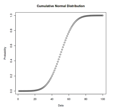
We can also plot the ECDF using the plot() function:

Output

Example 2: ECDF of Normally distributed data

Suppose we have a dataset of 100 observations that follows a normal distribution with a mean 0 and a standard deviation of 1. We want to compute the ECDF of this dataset and plot it.

1. Generate the data

We generate a dataset of 100 observations that follows a normal distribution with mean 0 and standard deviation 1. In R, we can use the rnorm() function to generate random normal data:

Here, we set the random seed to ensure reproducibility and generate 100 random numbers from a normal distribution with a mean of 0 and a standard deviation of 1. The resulting data object is a vector of length 100.

2. Compute the ECDF values

For each value of x, we want to compute the estimated probability that a data point in the dataset is less than or equal to x. We can compute the ECDF values manually using a for loop or using ecdf() function.

Output:

3. Check with ecdf() function identical or not

Output:

TRUE

4. Compute the cumulative normal distribution with new data

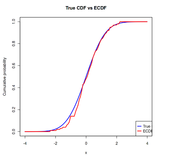
First, we define a sequence of values for x. For each value of x, we want to compute the true probability that a standard normal random variable is less than or equal to x. This can be done using the standard normal CDF and use the pnorm() function to compute the true CDF values for each value of x. we use the same sample mean and standard deviation here also.

Output:

5. Compute ecdf for x using the function ecdf_fun() and Plot both cdf and ecdf on same plot

We can plot the true CDF values and ECDF values on the same plot to visualize how closely they match. Here, we use the plot() function to create a line plot with x-values from -4 to 4 and y-values corresponding to the true CDF values in blue and the ECDF values in red. We also add a legend to the plot to distinguish between the two lines.

Output:

We first generate the normal data using the rnorm() function. Then, we compute the sample mean and standard deviation using the mean() and sd() functions. We then define a sequence of values for x and use the pnorm() function to compute the true CDF values for each value of x. We also compute the ECDF manually using a for loop and the sum() function. Finally, we plot both the true CDF.