How to Calculate Log-Linear Regression in R?

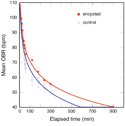
Logarithmic regression is a sort of regression that is used to simulate situations in which growth or decay accelerates quickly initially and then slows down over time. The graphic below, for example, shows an example of logarithmic decay:

The relationship between a predictor variable and a response variable could be properly described in this type of case utilizing logarithmic regression. A logarithmic regression model's equation looks like this:

where:

• y: The variable of response
• x: The regression coefficients that characterize the link between x and y are the predictor variables a, b.

Stepwise Implementation

Step 1: Gather the Data:

To begin, let's generate some fictitious data for two variables: x and y:

Step 2: Make the Data Visual:

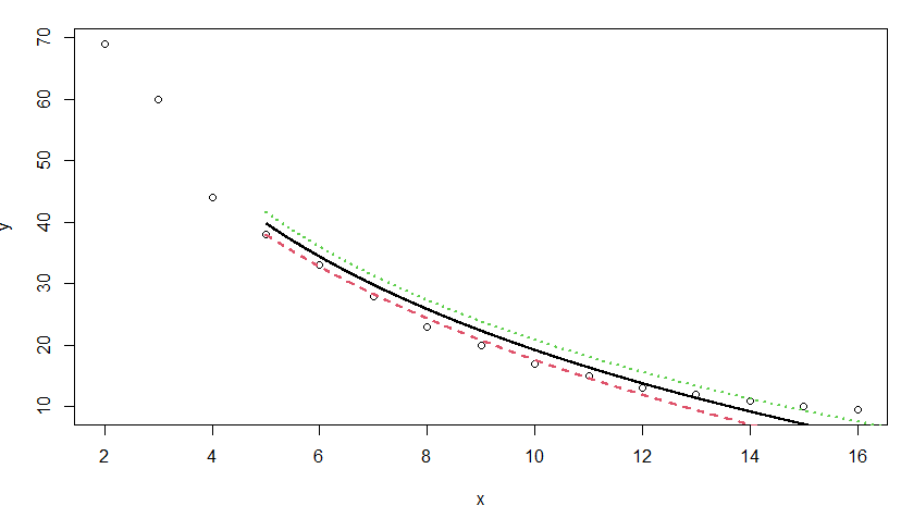
Let's now make a short scatterplot to show the relationship between x and y:

plot(x, y)

We can observe from the figure that there is a definite logarithmic decay pattern between the two variables. The value of the response variable, y, falls rapidly initially, then gradually diminishes with time. As a result, using a logarithmic regression equation to characterize the connection between the variables appears to be a decent approach.

Step 3: Create a Logarithmic Regression Model:

The lm() function will then be used to fit a logarithmic regression model with the natural log of x as the predictor variable and y as the response variable.

Call:

lm(formula = y ~ log(x))

Residuals:

   Min     1Q Median     3Q    Max 

-2.804 -1.972 -1.341  1.915  5.053 

Coefficients:

            Estimate Std. Error t value Pr(>|t|)    

(Intercept)   87.591      2.462   35.58 2.43e-14 ***

log(x)       -29.713      1.155  -25.72 1.56e-12 ***

---

Signif. codes:  0 ‘***’ 0.001 ‘**’ 0.01 ‘*’ 0.05 ‘.’ 0.1 ‘ ’ 1

Residual standard error: 2.69 on 13 degrees of freedom

Multiple R-squared:  0.9807, Adjusted R-squared:  0.9792 

F-statistic: 661.6 on 1 and 13 DF,  p-value: 1.557e-12

The model's overall F-value is 828.2, and the accompanying p-value is exceptionally low (3.702e-13), indicating that the model as a whole is beneficial. We can see from the coefficients in the output table that the fitted logarithmic regression equation is:

y = 63.1686 – 20.1987 ln (x)

Based on the value of the predictor variable, x, we can use this equation to predict the responder variable, y. For example, if x equals 12, we may anticipate that y equals 12.87:

y = 63.1686-20.1987 * ln(12) = 12.87

Note: You can use this online Logarithmic Regression Calculator to calculate the logarithmic regression equation for a given predictor and response variable.

Step 4: Create a visual representation of the Logarithmic Regression Model:

Finally, we can plot the data to see how well the logarithmic regression model matches the data:

Output: