 |
VOOZH | about |
|
VOOZH | about |
R Markdown is a file format for making dynamic and static documents with R. You can create an R Markdown file to save, organize and document your analysis using code chunks and comments. It is important to create an R Markdown file to have good communication between your team about analysis, you can create an R Markdown file to summarize your visuals to stakeholders. R Markdown documents are written in Markdown. Markdown is a syntax for formatting plain text files. It is also used to create rich format text in your document.
Documenting your work makes it easy to share your analysis with anyone, R Markdown lets you create a record of your analysis, conclusions, and decisions in a document. It binds together your code and your report so you can share every step of your analysis. R Markdown documents will help stakeholders and team members understand what you did in your analysis to reach your conclusions. We also have an interactive option called R Notebook that lets the user run their code and show the graphs and charts that visualize the code. R Markdown lets you convert files into other formats like HTML, PDF, Word documents, slide presentations, and dashboards also.
As we know R Markdown is a great tool for documenting your analysis, it is very easy to create and run R Markdown.
To create R Markdown Open R Studios in the menu bar, and click File -> New File -> R Markdown...
Syntax | Set Off |
| *italics* and _italics_ | change font to italic |
| **bold** and __bold__ | change font to bold |
| superscript^2^ | superscript2 |
| ~~strikethrough~~ | strikes off the text |
| # Header 1 | Big Header |
| ## Header 2 | Decrease the size of the Header than the Header! |
| inline equation: $A = \pi*r^{2}$ | inline equation: A = π * r2 |
| image:  | insert image in R Markdown from the specified path |
YAML header contains metadata of R markdown. Begins and end the header with a line of three dashes(---). You can change the information in this section at any time by adding text or by overriding the current text.
The output value gives which type of file will build from your .rmd file
Output Value | File Type |
| output: github_document | creates a Github document |
| output: html_document | HTML file(web page).html |
| output: pdf_document | pdf document.pdf |
| output: word_document | word document.docx |
| output: beamer_presentation | beamer slideshow |
| output: ioslides_presentation | slides slideshow |
The next part with gray background in R Markdown is the code chunk. We can run code chunks at any time.
RStudio automatically adds to the notebook with this formatted default code chunk. Code chunk starts with delimiter ` ` ` {r} and ends with ` ` `
There are two ways to add code chunks into an R Markdown document, you can press Ctrl + Alt + I(for windows) or Cmd + Option + I(for mac). Or you can use the Add Chunk command in the editor toolbar. In the default code section, we find "knitr" it is an R package with lightweight APIs designed to give users full control of the output format, it is used fully when you render your R Markdown document. We have different options in "knitr" package
Option | Default value | Effect |
eval | TRUE | evaluate the code and include its result if it is set to true |
echo | TRUE | display code along with its results if it is set to true |
warning | TRUE | display warnings |
message | TRUE | display messages |
tidy | FALSE | reformat code in a tidy way when displaying it |
error | FALSE | display errors |
cache | FALSE | cache results for future renders |
For example to add a code chunk,
Ctrl + Alt + I.
Output:
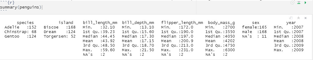
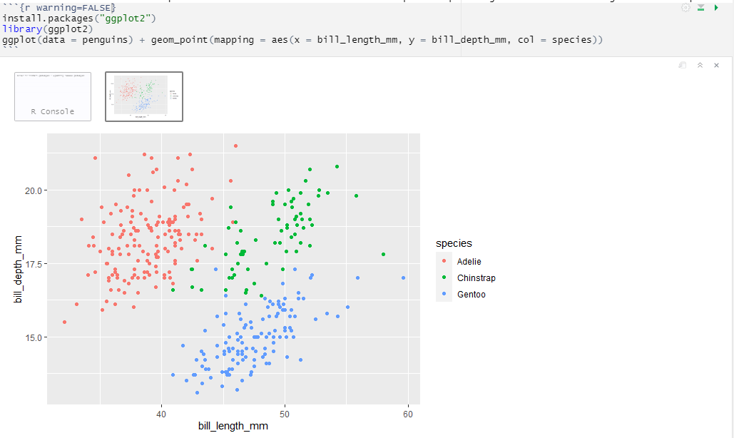
Now we will try to draw some plots by adding code in the R Markdown document.
Output:
You can run your R Markdown in two ways:
When you render your file, you can preview how it will look in the format you selected. Execute each code chunk and insert the result into your report and save the output file in your working directory.