Neural Networks Using the R nnet Package

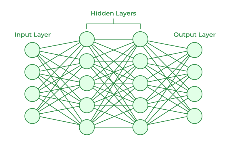
A neural network is a computational model inspired by the structure and function of the human brain. It consists of interconnected nodes, called neurons, organized into layers. The network receives input data, processes it through multiple layers of neurons, and produces an output or prediction.

The basic building block of a neural network is the neuron, which represents a computational unit. Each neuron takes input from other neurons or from the input data, performs a computation, and produces an output. The output of a neuron is typically determined by applying an activation function to the weighted sum of its inputs.

A neural network typically consists of three types of layers:

1. Input Layer: This layer receives the input data and passes it to the next layer. Each neuron in the input layer corresponds to a feature or attribute of the input data.
2. Hidden Layers: These layers are placed between the input and output layers and perform computations on the data. Each neuron in a hidden layer takes input from the neurons in the previous layer and produces an output that is passed to the neurons in the next layer. Hidden layers enable the network to learn complex patterns and relationships in the data.
3. Output Layer: This layer produces the final output or prediction of the neural network. The number of neurons in the output layer depends on the nature of the problem. For example, in a binary classification problem, there may be one neuron representing the probability of one class and another neuron representing the probability of the other class. In a regression problem, there may be a single neuron representing the predicted numerical value.

👁 Neural-Networks-Architecture.pngGeeksforgeeks

During training, the neural network adjusts the weights and biases associated with each neuron to minimize the difference between the predicted output and the true output. This is achieved using an optimization algorithm, such as gradient descent, which iteratively updates the weights and biases based on the error or loss between the predicted and actual outputs.

The choice of activation function for the neurons is important, as it introduces non-linearity into the network. Common activation functions include the sigmoid function, ReLU (Rectified Linear Unit), and softmax. The activation function determines the output range of a neuron and affects the network's ability to model complex relationships.

Neural networks can be applied to a wide range of tasks, including classification, regression, image recognition, natural language processing, and more. They have shown great success in many domains, but their performance depends on the quality and size of the training data, the network architecture, and the appropriate selection of hyperparameters.

nnet Package in R

The "nnet" package in R is a widely used package that provides functions for building and training neural networks. It stands for "Feed-Forward Neural Networks and Multinomial Log-Linear Models."

The "nnet" package primarily focuses on feed-forward neural networks, which are a type of artificial neural network where the information flows in one direction, from the input layer to the output layer. These networks are well-suited for tasks such as classification and regression.

The package offers the nnet() function, which is the main function used to create and train neural networks. It allows you to specify the network architecture, including the number of layers, the number of neurons in each layer, and the activation function to be used. The default activation function is the logistic sigmoid function, but you can also choose other options, such as the hyperbolic tangent function.

The main features of the nnet package are explained below:

1. Neural Network Architecture: The nnet the function is the primary function used to create a neural network model. It allows you to specify the neural network's architecture, including the number of hidden layers, the number of nodes in each layer, and the activation function to be used.
2. Model Training: The nnet the function also performs the training of the neural network model. It uses an optimization algorithm, such as the backpropagation algorithm, to iteratively adjust the network weights based on the training data.
3. Model Prediction: Once the neural network model is trained, you can use the predict function to make predictions on new data. It takes the trained model and the new data as input and returns the predicted values or class probabilities depending on the type of task.
4. Model Evaluation: Evaluation metrics, such as accuracy, confusion matrix, precision, recall, and F1-score, can be calculated using appropriate functions from other packages like caret or yardstick.

Example 1: Classification

To use the R nnet package for classification with user-defined data.

Step 1: Prepare the data

In this step, we generate a sample dataset for classification. It includes two numeric features x1 and x2, and a target variable class. We generate random values for x1 and x2 using the rnorm() function. The class variable is assigned as "Class A" if x1 + x2 is greater than 0, and "Class B" otherwise. The features and target variable are combined into a data frame my_data. The target variable class is converted to a factor using as.factor().

Let's break down each line of code:

1. set.seed(123): This sets the seed for random number generation, ensuring the of reproducibility of the results. Setting the same seed will generate the same random numbers each time the code is run.
2. n <- 200: This assigns the number of observations we want to generate in our dataset. In this case, we generate 200 observations.
3. x1 <- rnorm(n, mean = 0, sd = 1): The rnorm() the function is used to generate random numbers from a normal distribution. It takes the arguments n (number of observations), mean (mean of the distribution), and sd (standard deviation of the distribution). Here, we generate n random numbers from a normal distribution with a mean of 0 and a standard deviation of 1 and assign them to the variable x1.
4. x2 <- rnorm(n, mean = 0, sd = 1): Similarly, we generate n random numbers from a normal distribution with mean 0 and standard deviation 1, and assign them to the variable x2.
5. class <- ifelse(x1 + x2 > 0, "Class A", "Class B"): We use the ifelse() function to create a target variable class based on a condition. If the sum of x1 and x2 is greater than 0, we assign "Class A" to the , otherwise "Class B" is assigned. This creates two distinct classes based on a linear separation.
6. my_data <- data.frame(x1, x2, class): We combine the features x1, x2, and the target variable class into a data frame called my_data. This creates our dataset with the features and corresponding target values.
7. my_data$class <- as.factor(my_data$class): Finally, we convert the target variable class to a factor using the as.factor() function. This is necessary for classification models, as factors represent categorical variables with levels that can be used for classification purposes.

Step 2: Split the Data

In this step, we split the data into training and testing sets. We load the caret package. The createDataPartition() the function is used to randomly split the data based on the target variable my_data$class. We specify p = 0.7 to allocate 70% of the data for training and 30% for testing. The list = FALSE parameter ensures that the output is a vector of indices. The training set is assigned to train_data, and the testing set is assigned to test_data.

Let's break down each line of code:

1. library(caret): We load the caret package, which provides useful functions for data splitting, modeling, and evaluation.
2. set.seed(123): This sets the seed for random number generation, ensuring the reproducibility of the results. Setting the same seed will generate the same random numbers each time the code is run.
3. split <- createDataPartition(my_data$class, p = 0.7, list = FALSE): The createDataPartition() function from the caret package is used to split the data. It takes the target variable my_data$class and splits the data into two groups based on the proportion specified by p. Here, we specify p = 0.7, which means that 70% of the data will be allocated for training. The list = FALSE parameter ensures that the output is a vector of indices.
4. train_data <- my_data[split, ]: We create the training dataset by subsetting my_data using the indices obtained from the split variable. This assigns the rows corresponding to the indices to train_data.
5. test_data <- my_data[-split, ]: We create the testing dataset by subsetting my_data using the negative of the indices obtained from the split variable. This assigns the rows not included in the training set to test_data.
6. train_data$class <- factor(train_data$class, levels = levels(my_data$class)): The factor() the function is used to convert the class variable in the train_data dataset to a factor variable. We specify the levels argument to be the same as the levels of the original my_data$class variable. This ensures that the levels train_data$class match the levels in the original dataset.
7. test_data$class <- factor(test_data$class, levels = levels(my_data$class)): Similarly, the class variable in the test_data dataset is converted to a factor variable using the factor() function. The levels argument is set to the levels of the original my_data$class variable to ensure consistency

By performing this step, we ensure that both the training and testing datasets have the same levels for the target variable. This is important for consistent modeling and evaluation.

Step 3: Model Training

In this step, we train the neural network using the nnet() function from the nnet package. We specify the formula class ~ x1 + x2, which represents the relationship between the features x1 and x2 the target variable class. The data the parameter is set to the training data train_data. The size parameter specifies the number of nodes in the hidden layer, set to 5 in this example. The maxit parameter sets the maximum number of iterations for the training process, set to 1000.

Output:

weights: 21
initial value 101.155606 
iter 10 value 0.969817
iter 20 value 0.000362
final value 0.000089 
converged

Let's break down each line of code:

1. library(nnet): We load the nnet package, which provides functions for building and training neural networks.
2. formula <- class ~ x1 + x2: We define the formula that represents the relationship between the features x1 and x2 and the target variable class. The formula has the format target_variable ~ predictor_variable1 + predictor_variable2 + .... In this case, we specify class ~ x1 + x2, indicating that class is the target variable, and x1 and x2 are the predictor variables.
3. model <- nnet(formula, data = train_data, size = 5, maxit = 1000): We use the nnet() function to train the neural network model. The function takes several arguments:
   • formula: The formula representing the relationship between the features and the target variable.
   • data: The training data, which is train_data in this case.
   • size: The number of nodes in the hidden layer of the neural network. Here, we set it to 5, but you can choose a different value based on your specific problem.
   • maxit: The maximum number of iterations for the training process. We set it to 1000, but you can adjust it based on the convergence of the model.

The nnet() function fits a neural network model to the training data using the specified formula and parameters. The resulting model is stored in the model object.

In summary, Step 3 uses the nnet() function from the nnet package to train a neural network model. It takes the formula representing the relationship between the features and the target variable, the training data, and parameters such as the number of nodes in the hidden layer and the maximum number of iterations.

Step 4: Model Evaluation

In this step, we evaluate the trained model using the testing data. The predict() function is used to make predictions on the test_data using the trained model. The newdata the parameter specifies the data to predict on. We set type = "class" to obtain class predictions. Next, we use the confusionMatrix() function from the caret package to create a confusion matrix. It takes the predicted values predictions and the actual values test_data$class as inputs. The confusionMatrix() the function computes various evaluation metrics such as accuracy, precision, recall, etc. Finally, we extract the accuracy from the confusion_matrix using the $overall attribute and print it using the print() function.

Output:

Confusion Matrix and Statistics
 Reference
Prediction Class A Class B
 Class A 31 0
 Class B 0 28

 Accuracy : 1 
 95% CI : (0.9394, 1)
 No Information Rate : 0.5254 
 P-Value [Acc > NIR] : < 2.2e-16 

 Kappa : 1 

 Mcnemar's Test P-Value : NA 

 Sensitivity : 1.0000 
 Specificity : 1.0000 
 Pos Pred Value : 1.0000 
 Neg Pred Value : 1.0000 
 Prevalence : 0.5254 
 Detection Rate : 0.5254 
 Detection Prevalence : 0.5254 
 Balanced Accuracy : 1.0000 

 'Positive' Class : Class A 

Let's break down each line of code:

1. library(caret): We load the caret package, which provides functions for model evaluation and performance metrics.
2. predictions <- predict(model, newdata = test_data, type = "class"): We use the predict() function to make predictions on the testing data using the trained model. The function takes several arguments:
   • model: The trained neural network model obtained from Step 3.
   • newdata: The data on which we want to make predictions. Here, we use test_data, which is the testing dataset.
   • type: The type of prediction we want. Since this is a classification problem, we set it to "class" to obtain class predictions.
   The predicted class labels are stored in the predictions variable.
3. confusion_matrix <- confusionMatrix(predictions, test_data$class): We use the confusionMatrix() function from the caret package to create a confusion matrix. The function takes the predicted values (predictions) and the actual values (test_data$class) as inputs. It computes various evaluation metrics such as accuracy, precision, recall, etc., and returns a confusionMatrix object. The resulting confusion matrix is stored in the confusion_matrix variable.
4. accuracy <- confusion_matrix$overall["Accuracy"]: We extract the accuracy from the confusion_matrix object using the $overall attribute. The $overall attribute contains overall performance metrics and "Accuracy" specifies the accuracy value.
5. print(paste("Accuracy:", accuracy)): We print the accuracy value using the print() function. The paste() function is used to concatenate the string "Accuracy:" with the actual accuracy value.

[1] "Accuracy: 1"

In summary, Step 4 evaluates the trained neural network model by making predictions on the testing data and computing the accuracy. The predict() a function is used to obtain class predictions, the confusionMatrix() the function creates a confusion matrix to evaluate model performance, and the accuracy value is extracted from the confusion matrix and printed.

This is how we can perform the classification of data using nnet package in R.

Example 2: Regression

Here's an example of performing regression using the nnet package in R on a created dataset.

Step 1: Prepare the Data

In this step, a sample dataset for regression is created by generating random predictor variables and a response variable. The data is combined into a data frame, and the response variable is converted to a factor.

Here's an explanation of each line of code:

1. set.seed(123): Sets the seed for reproducibility. By setting a seed, the generated random numbers will be the same each time the code is run.
2. n <- 200: Specifies the number of observations. In this case, we have 200 observations.
3. x1 <- rnorm(n, mean = 0, sd = 1): Generates random values for the predictor variable x1 from a normal distribution. The rnorm() function generates n random numbers with a mean of 0 and a standard deviation of 1.
4. x2 <- rnorm(n, mean = 0, sd = 1): Generates random values for the predictor variable x2 using the same approach as in the previous line.
5. y <- 2*x1 + 3*x2 + rnorm(n, mean = 0, sd = 0.5): Generates the response variable y based on a linear relationship with noise. It combines the predictor variables x1 and x2 with weights of 2 and 3, respectively. The rnorm() function generates random noise with a mean of 0 and a standard deviation of 0.5.
6. my_data <- data.frame(x1, x2, y): Combines the predictor variables x1, x2, and the response variable y into a data frame called my_data. Each variable becomes a column in the data frame.

These steps generate a synthetic dataset with two predictor variables x1 and x2, and a response variable y that follows a linear relationship with some added noise.

Step 2: Split the Data

The dataset is split into training and testing sets using the createDataPartition() function from the caret package. The data is divided based on a specified proportion, and the resulting subsets are assigned to train_data and test_data.

Here's an explanation of each line of code:

1. library(caret): Loads the caret package, which provides functions for data splitting and preprocessing.
2. set.seed(123): Sets the seed for reproducibility. This ensures that the data split will be the same each time the code is run.
3. split <- createDataPartition(my_data$y, p = 0.7, list = FALSE): Uses the createDataPartition() function from the caret package to split the data into training and testing sets. The createDataPartition() function takes the response variable my_data$y and splits the data based on the specified proportion (p = 0.7, meaning 70% for training and 30% for testing). The list = FALSE parameter indicates that the result should be returned as a vector of indices.
4. train_data <- my_data[split, ]: Assigns the training data by subsetting my_data using the indices obtained from the split vector. This extracts the rows corresponding to the indices in split and assigns them to train_data.
5. test_data <- my_data[-split, ]: Assigns the testing data by subsetting my_data using the negative indices of split. This extracts the rows not included in split and assigns them to test_data.

By splitting the data into training and testing sets, we can use the training data to train the model and evaluate its performance on the testing data.

Step 3: Model Training

The nnet package is loaded, and a neural network model is trained using the nnet() function. The model is trained using the training data, and the formula specifies the relationship between the response variable and predictor variables. Additional parameters like the number of hidden nodes and maximum iterations are set.

Output:

# weights: 21
initial value 1733.825618 
iter 10 value 325.524695
iter 20 value 125.208619
iter 30 value 38.444341
iter 40 value 31.529450
iter 50 value 30.506822
iter 60 value 28.372888
iter 70 value 27.656570
iter 80 value 27.594377
iter 90 value 27.562448
iter 100 value 27.517448
iter 110 value 27.495839
iter 120 value 27.338752
iter 130 value 27.241432
iter 140 value 27.226825
iter 150 value 27.164398
iter 160 value 27.148384
iter 170 value 27.107991
iter 180 value 27.104630
iter 190 value 27.100312
iter 200 value 27.087177
iter 210 value 27.055133
iter 220 value 27.043583
iter 230 value 27.036930
iter 240 value 27.029102
iter 250 value 27.026189
iter 260 value 27.025619
iter 270 value 27.025371
iter 280 value 27.024260
iter 290 value 27.023630
iter 300 value 27.021395
iter 310 value 27.019450
iter 320 value 27.018149
iter 330 value 27.017640
iter 340 value 27.012681
iter 350 value 26.998627
iter 360 value 26.994418
iter 370 value 26.993394
iter 380 value 26.990601
iter 390 value 26.989293
iter 400 value 26.989118
iter 410 value 26.986376
iter 420 value 26.985672
iter 430 value 26.983334
iter 440 value 26.981814
iter 450 value 26.981003
iter 460 value 26.978700
iter 470 value 26.978033
iter 480 value 26.977101
iter 490 value 26.975884
iter 500 value 26.973281
iter 510 value 26.972808
iter 520 value 26.967412
iter 530 value 26.965805
iter 540 value 26.964680
iter 550 value 26.962324
iter 560 value 26.961902
iter 570 value 26.961771
iter 580 value 26.961526
iter 590 value 26.958141
iter 600 value 26.953665
iter 610 value 26.950821
iter 620 value 26.949362
iter 630 value 26.945554
iter 640 value 26.940451
final value 26.940071 
converged

Here's an explanation of the code:

1. library(nnet): Loads the nnet package, which provides functions for training neural network models.
2. model <- nnet(y ~ x1 + x2, data = train_data, size = 5, maxit = 1000, linout = TRUE): Trains the neural network model for regression using the nnet() function.
   • y ~ x1 + x2: Specifies the formula representing the relationship between the response variable y and the predictor variables x1 and x2.
   • data = train_data: Specifies the training dataset from which the model will learn.
   • size = 5: Specifies the number of nodes in the single hidden layer of the neural network. In this case, the hidden layer will have 5 nodes.
   • maxit = 1000: Specifies the maximum number of iterations or epochs for which the neural network will be trained. The model will stop training if it reaches this maximum number of iterations before convergence.
   • linout = TRUE: Sets the output function of the neural network to be linear, indicating that the model is trained for regression instead of classification. By default, the nnet() function assumes a logistic output function for classification tasks, but here we explicitly set it to linear for regression.

The trained model is stored in the model object and can be used for making predictions on new data.

Step 4: Model Evaluation

Predictions are made on the test data using the trained model and the predict() function. The caret the package is loaded, and the Root Mean Squared Error (RMSE) between the predicted and actual values is calculated using the caret::RMSE() function. The RMSE serves as a measure of the model's performance in regression tasks.

Here's an explanation of each line of code:

1. predictions <- predict(model, newdata = test_data): Uses the trained model to make predictions on the test data. The predict() function takes the trained model and the new data (test_data) as input and returns the predicted values based on the model.
2. library(caret): Loads the caret package, which provides functions for model evaluation and performance metrics.
3. rmse <- caret::RMSE(predictions, test_data$y): Calculates the Root Mean Squared Error (RMSE) between the predicted values (predictions) and the actual response values (test_data$y). The caret::RMSE() the function is used to compute the RMSE.
4. print(paste("Root Mean Squared Error (RMSE):", rmse)): Prints the calculated RMSE value. The paste() function is used to concatenate the string "Root Mean Squared Error (RMSE):" with the actual RMSE value (rmse), and the result is printed to the console.

[1] "Root Mean Squared Error (RMSE): 0.572527937783828"

The RMSE is a common metric used to evaluate the performance of regression models. It measures the average magnitude of the residuals (the differences between the predicted and actual values) and provides an overall assessment of the model's predictive accuracy.

In this way,the regression can be performed using the nnet package in R

To conclude we have learned how to perform classification and regression using the nnet package in R.