SARIMA in R

SARIMA (Seasonal Autoregressive Integrated Moving Average) is an extension of the ARIMA model that incorporates seasonality into the model. It’s a powerful tool for modeling and forecasting time series data that exhibit both trend and seasonality.

What is SARIMA?

SARIMA is a variant of the ARIMA model that takes into account both non-seasonal and seasonal components in a time series. It is designed to capture data that shows patterns at regular intervals, such as quarterly sales or monthly weather data.

The SARIMA model is often written as:

SARIMA(p,d,q)(P,D,Q)m​

where,

• p,d,q are the non-seasonal ARIMA terms.
• P,D,Q are the seasonal ARIMA terms.
• m is the number of periods in each seasonal cycle.

• p: The number of autoregressive terms.
• d: The number of differences needed to make the time series stationary.
• q: The number of moving average terms.
• P: The number of seasonal autoregressive (SAR) terms.
• D: The number of seasonal differences.
• Q: The number of seasonal moving average (SMA) terms.
• m: The length of the seasonal cycle.

Why Use SARIMA?

• Handles Seasonality: It effectively models data with seasonal patterns.
• Flexibility: The combination of seasonal and non-seasonal parameters allows it to adapt to various datasets.
• Good Forecasting Performance: SARIMA can provide accurate forecasts when the underlying data patterns are appropriately modeled.

Now we implement SARIMA in R Programming Language.

Step 1: Install and Load Required Packages

First, install and Load the necessary packages.

Step 2: Create Synthetic Monthly Sales Data

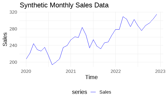
Generate synthetic sales data for 36 months.

Output:

 Date Sales
1 2020-01-01 207.3952
2 2020-02-01 221.0187
3 2020-03-01 244.5871
4 2020-04-01 230.0256
5 2020-05-01 226.2929
6 2020-06-01 235.1506

Step 3: Convert to Time Series Format

Convert the data frame into a time series object.

Step 4: Visualize the Data

Plot the synthetic sales data to visualize trends.

Output:

Step 5: Check for Stationarity

Perform the Augmented Dickey-Fuller test to check for stationarity.

Output:

 Augmented Dickey-Fuller Test

data: ts_data
Dickey-Fuller = -5.3005, Lag order = 3, p-value = 0.01
alternative hypothesis: stationary

Step 6: Identify Model Parameters

Now find suitable model parameters.

Output:

Series: ts_data 
ARIMA(0,0,0)(1,1,0)[12] with drift 

Coefficients:
 sar1 drift
 -0.8392 2.9958
s.e. 0.0854 0.1095

sigma^2 = 83.1: log likelihood = -93.36
AIC=192.71 AICc=193.91 BIC=196.25

Training set error measures:
 ME RMSE MAE MPE MAPE MASE
Training set -0.4441953 7.126158 4.467821 -0.2139526 1.667343 0.1240441
 ACF1
Training set 0.1815494

Step 7: Fit the SARIMA Model

Fit the SARIMA model with chosen parameters.

Output:

Series: ts_data 
ARIMA(1,1,1)(1,1,1)[12] 

Coefficients:
 ar1 ma1 sar1 sma1
 0.0267 -0.7219 -0.8417 -0.0275
s.e. 0.3068 0.2199 NaN NaN

sigma^2 = 97.05: log likelihood = -91.09
AIC=192.18 AICc=195.71 BIC=197.86

Training set error measures:
 ME RMSE MAE MPE MAPE MASE
Training set 0.3929868 7.156714 4.692756 0.07424912 1.739757 0.1302892
 ACF1
Training set -0.02246882

Step 8: Predict the data

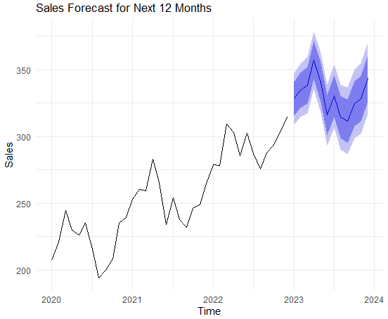
Generate forecasts for the next 12 months.

Step 9: Plot the Forecasted Values

Visualize the forecasted values with confidence intervals.

Output:

Step 10: Evaluate Model Performance

Check the accuracy of the model's predictions.

Output:

 ME RMSE MAE MPE MAPE MASE
Training set 0.3929868 7.156714 4.692756 0.07424912 1.739757 0.1302892
 ACF1
Training set -0.02246882

Applications and Use Cases of SARIMA

• Sales Forecasting: Businesses use SARIMA to predict future sales based on historical data, helping with inventory management and production planning.
• Weather Forecasting: Meteorologists employ SARIMA to model and forecast temperature, rainfall, and other climate variables, which often exhibit seasonal trends.
• Financial Market Analysis: In finance, SARIMA can analyze and predict stock prices, interest rates, and economic indicators, aiding investment decisions.
• Energy Consumption Forecasting: Utilities use SARIMA to estimate future energy demands, allowing for better resource allocation and grid management.
• Healthcare Data Analysis: SARIMA helps analyze patient admission rates, disease outbreaks, and other healthcare-related time series, aiding in resource planning and management.

Advantages of SARIMA

• Ideal for datasets with clear seasonal patterns.
• Can be customized with different parameters to fit various types of data.
• When properly configured, SARIMA can produce accurate forecasts.

Limitations of SARIMA

• SARIMA may not perform well with datasets that have complex, nonlinear relationships.
• Requires sufficient historical data to effectively model and forecast.
• Can be influenced by outliers, which may distort the forecasts.

Conclusion

SARIMA is a powerful statistical tool for forecasting time series data that exhibit both trends and seasonality. By combining autoregressive and moving average components, along with seasonal adjustments, it offers flexibility and accuracy in modeling complex datasets. Understanding how to implement SARIMA in R enhances the ability to derive insights from time series data, making it an invaluable resource for data analysts, researchers, and business professionals.