Exponential Distribution in R Programming - dexp(), pexp(), qexp(), and rexp() Functions

The Exponential Distribution is a continuous probability distribution that models the time between independent events occurring at a constant average rate. It is widely used in fields like reliability analysis, queuing theory, and survival analysis. The exponential distribution is a special case of the Gamma distribution.

In R, there are four built-in functions to work with the exponential distribution:

• dexp() : Computes the Probability Density Function (PDF).
• pexp() : Computes the Cumulative Distribution Function (CDF).
• qexp() : Computes the Quantile Function (inverse of the CDF).
• rexp() : Generates random numbers that follow an exponential distribution.

Mathematical Understanding

A random variable X is said to follow an exponential distribution with rate parameter λ (lambda) if:

• Mean of the distribution is:
• Variance of the distribution is:

1. The Probability Density Function (PDF) is defined as:

Where:

• is the rate parameter.
• is the time until the next event occurs.

Similarly ,

2. The Cumulative Distribution Function (CDF) is defined as :

Where:

• is the rate parameter.
• is the time until the next event occurs.

3. The Quantile Function (Inverse CDF) is defined as :

Where:

• : A probability value in the range (0,1)(0, 1)(0,1)
• is the rate parameter.

Implementation of Different Exponential Distribution functions in R

We will now , implement the four function available in R programming language and understands there working and interpretation.

1. dexp() Function

The dexp() function returns the corresponding values of the exponential density for an input vector of quantiles. This function calculates the Probability Density Function (PDF) of the exponential distribution at each point in x, given the specified rate. It is used to understand how the probability is distributed over the range of possible values.

Syntax:

dexp(x_dexp, rate)

Parameters:

• x : A numeric vector of quantiles (the input values for which the density is calculated).
• rate : The rate parameter () of the exponential distribution( Must be positive).

Example: 

We are generating a sequence of values from 1 to 10 and computing their exponential probability densities using a rate of 5. Then, we plot the resulting density values to visualize the shape of the exponential distribution.

Output:

2. pexp() Function

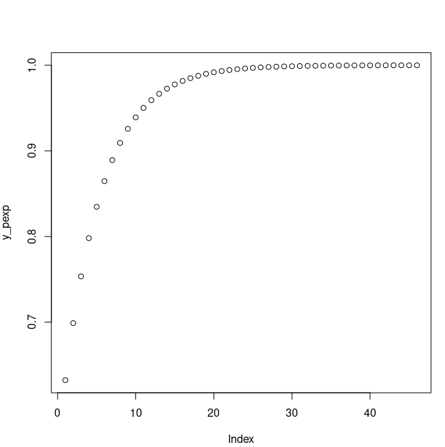
The pexp() function returns the corresponding values of the exponential cumulative distribution function for an input vector of quantiles. This function computes the cumulative probability that a random variable drawn from an exponential distribution with the given rate is less than or equal to each value in x. It is useful for determining the probability of an event occurring within a certain time frame.

Syntax:

pexp(x_pexp, rate )

Parameters:

• x : A numeric vector of quantiles (the input values for which the cumulative probability is calculated).
• rate : The rate parameter () of the exponential distribution ( Must be positive).

Example:

We are creating a sequence of values from 1 to 10, then computing their cumulative probabilities using the exponential cumulative distribution function with a rate of 1. Finally, we plot the resulting CDF values to visualize how probability accumulates over time in an exponential distribution.

Output :

3. qexp() Function

The qexp() function in R returns the quantile function (inverse CDF) values of the exponential distribution for a given set of probabilities. This function calculates the quantile (inverse CDF) , the value x such that the probability of an exponentially distributed random variable being less than or equal to x is equal to p. It is used when you want to determine what value corresponds to a specific cumulative probability.

Syntax:

qexp(x_qexp, rate)

Parameters:

• p : A numeric vector of probabilities (values between 0 and 1).
• rate : The rate parameter (λ) of the exponential distribution ( Must be positive ).

Example:

We are generating a sequence of probabilities from 0 to 1, then using the exponential quantile function with a rate of 1 to find the corresponding quantile values. Finally, we plot these quantiles to visualize how values grow with increasing cumulative probability in an exponential distribution.

Output:

4. rexp() Function

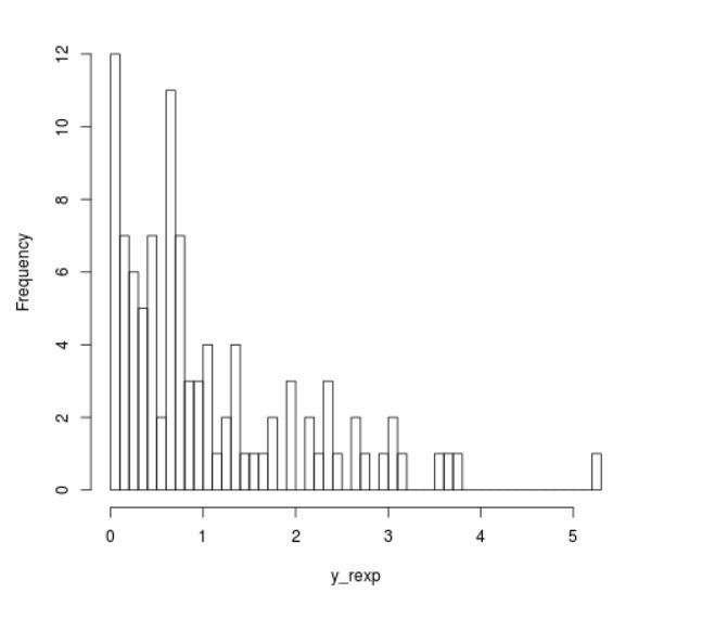
The rexp() function in R is used to generate random numbers that follow an exponential distribution with a specified rate. This function simulates random values from an exponential distribution defined by the given rate. It is commonly used in simulations, stochastic modeling, and random sampling where event timing is modeled using exponential behavior.

Syntax:

rexp(N, rate )

Parameters:

• n : Number of random values to generate.
• rate : The rate parameter (λ) of the exponential distribution ( Must be positive).

Example:

We are setting a random seed for reproducibility, then generating 100 random values from an exponential distribution with a rate of 1. Finally, we plot a histogram with 50 bins to visualize the distribution of the generated data.

Output:

In this article , we explored the different exponential distribution functions in R programming language and implemented the same with visualizations.