Geometric Distribution in R

The geometric distribution in R is one of the fundamental discrete probability distributions in statistics. It models the number of trials required to get the first success in a sequence of independent Bernoulli trials (i.e., trials with two possible outcomes: success and failure). In this article, we will explore the theory behind the geometric distribution, its probability mass function (PMF), cumulative distribution function (CDF), and its applications. We will also cover how to work with the geometric distribution in R with practical examples.

The geometric distribution in R arises when we perform a sequence of independent and identically distributed Bernoulli trials, where each trial has:

• Two possible outcomes Success (with probability p) and Failure (with probability 1−p).
• We are interested in the number of trials needed to get the first success.

Mathematically, the probability mass function (PMF) of a geometric distribution is given by:

Where:

• X is the random variable representing the number of trials needed for the first success.
• p is the probability of success in each trial.
• k is the number of trials (a positive integer).

Applications of the Geometric Distribution in R

The geometric distribution is useful in various real-world scenarios, such as:

• Modeling the number of times a gambler plays until they win.
• Estimating the number of inspections needed to find a defective product in quality control.
• Predicting the number of phone calls until the first one is answered.

Working with the Geometric Distribution in R

R provides built-in functions to handle the geometric distribution in R its including generating random samples, calculating probabilities, and plotting the distribution. Functions in R for the Geometric Distribution

1. dgeom(x, prob): Computes the probability mass function (PMF) at point x.
2. pgeom(q, prob): Computes the cumulative distribution function (CDF) up to q.
3. qgeom(p, prob): Computes the quantile function (inverse of the CDF) for a given probability p.
4. rgeom(n, prob): Generates nnn random variates from the geometric distribution with success probability prob.

Now we will discuss all the function in detail to calculate Geometric Distribution in R Programming Language.

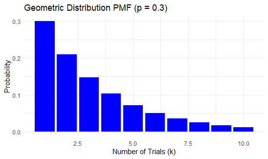
1: Calculate Probability Mass Function (PMF) using dgeom()

The dgeom() function computes the probability mass function (PMF), i.e., the probability of getting the first success on the k-th trial. Let’s compute and visualize the PMF for k=1,2,…,10 with p=0.3 (probability of success).

Output:

This plot shows the probabilities of getting the first success on each trial.

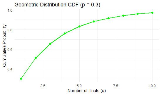
2: Calculate Cumulative Distribution Function (CDF) using pgeom()

The pgeom() function computes the cumulative probability of getting the first success on or before the q-th trial. Let’s calculate and plot the CDF for q=1,2,…,10 with p=0.3.

Output:

This plot shows the cumulative probability of getting the first success on or before each trial.

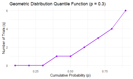
3: Calculate Quantile Function (Inverse CDF) using qgeom()

The qgeom() function calculates the number of trials qqq needed to achieve a given cumulative probability. Let’s compute the number of trials for different probabilities p=0.1,0.2,…,0.9 with p=0.3.

Output:

This plot shows how many trials are expected to get the first success for different cumulative probabilities.

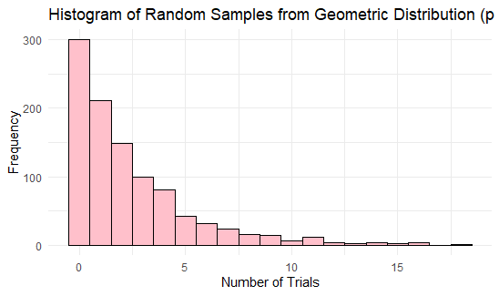
4: Random Sampling from Geometric Distribution using rgeom()

The rgeom() function generates random samples from a geometric distribution. Let’s generate 1000 random samples and visualize their distribution using a histogram.

Output:

This histogram shows the frequency distribution of the number of trials required to get the first success in 1000 random samples.