Regularization in R Programming

Regularization is a form of regression technique that shrinks or regularizes or constraints the coefficient estimates towards 0 (or zero). In this technique, a penalty is added to the various parameters of the model in order to reduce the freedom of the given model. The concept of Regularization can be broadly classified into:

• Ridge Regression
• Lasso Regression
• Elastic Net Regression

Implementation in R

In the R language, to perform Regularization we need a handful of packages to be installed before we start working on them. The required packages are 

• glmnet package for ridge regression and lasso regression
• dplyr package for data cleaning
• psych package in order to perform or compute the trace function of a matrix
• caret package

To install these packages we have to use the install.packages() in the R Console. After installing the packages successfully, we include these packages in our R Script using the library() command. To implement the Regularization regression technique we need to follow either of the three types of regularization techniques.

Ridge Regression

The Ridge Regression is a modified version of linear regression and is also known as L2 Regularization. Unlike linear regression, the loss function is modified in order to minimize the model's complexity and this is done by adding some penalty parameter which is equivalent to the square of the value or magnitude of the coefficient. Basically, to implement Ridge Regression in R we are going to use the "glmnet" package. The cv.glmnet() function will be used to determine the ridge regression. 

Example:

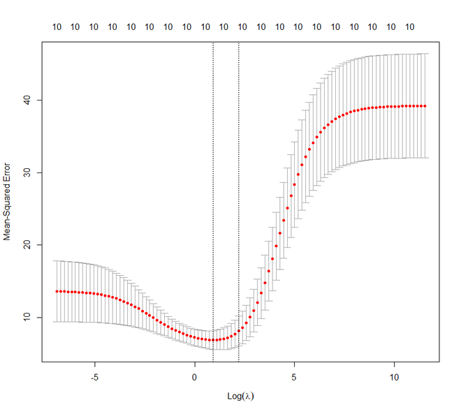
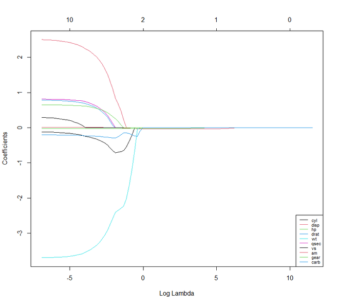
In this example, we will implement the ridge regression technique on the mtcars dataset for a better illustration. Our task is to predict the miles per gallon on the basis of other characteristics of the cars. We are going to use the set.seed() function to set seed for reproducibility. We are going to set the value of lambda in three ways:

• by performing 10 fold cross-validation
• based on the information derived
• optimal lambda based on both the criteria

Output:

Lasso Regression

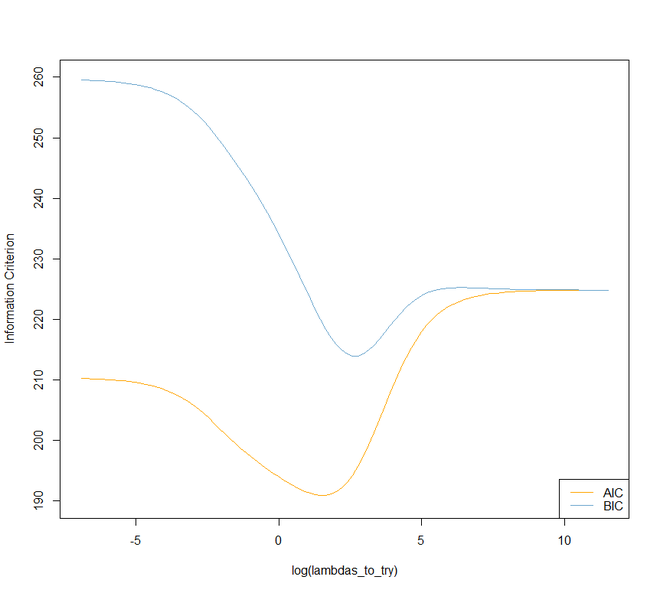
Moving forward to Lasso Regression. It is also known as L1 Regression, Selection Operator, and Least Absolute Shrinkage. It is also a modified version of Linear Regression where again the loss function is modified in order to minimize the model's complexity. This is done by limiting the summation of the absolute values of the coefficients of the model. In R, we can implement the lasso regression using the same "glmnet" package like ridge regression.

Example:

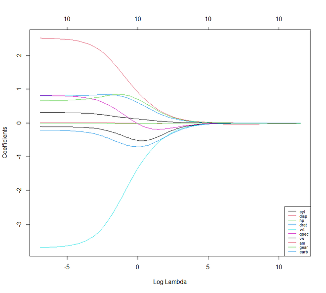
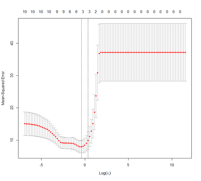
Again in this example, we are using the mtcars dataset. Here also we are going to set the lambda value like the previous example.

Output:

If we compare Lasso and Ridge Regression techniques we will notice that both the techniques are more or less the same. But there are few characteristics where they differ from each other.

• Unlike Ridge, Lasso can set some of its parameters to zero.
• In ridge the coefficient of the predictor that is correlated is similar. While in lasso only one of the coefficient of predictor is larger and the rest tends to zero.
• Ridge works well if there exist many huge or large parameters that are of the same value. While lasso works well if there exist only a small number of definite or significant parameters and rest tending to zero.

Elastic Net Regression

We shall now move on to Elastic Net Regression. Elastic Net Regression can be stated as the convex combination of the lasso and ridge regression. We can work with the glmnet package here even. But now we shall see how the package caret can be used to implement the Elastic Net Regression.

Example:

Output:

> print(y_hat_enet)
 Mazda RX4 Mazda RX4 Wag Datsun 710 Hornet 4 Drive Hornet Sportabout Valiant 
 2.13185747 1.76214273 6.07598463 0.50410531 -3.15668592 0.08734383 
 Duster 360 Merc 240D Merc 230 Merc 280 Merc 280C Merc 450SE 
 -5.23690809 2.82725225 2.85570982 -0.19421572 -0.16329225 -4.37306992 
 Merc 450SL Merc 450SLC Cadillac Fleetwood Lincoln Continental Chrysler Imperial Fiat 128 
 -3.83132657 -3.88886320 -8.00151118 -8.29125966 -8.08243188 6.98344302 
 Honda Civic Toyota Corolla Toyota Corona Dodge Challenger AMC Javelin Camaro Z28 
 8.30013895 7.74742320 3.93737683 -3.13404917 -2.56900144 -5.17326892 
 Pontiac Firebird Fiat X1-9 Porsche 914-2 Lotus Europa Ford Pantera L Ferrari Dino 
 -4.02993835 7.36692700 5.87750517 6.69642869 -2.02711333 0.06597788 
 Maserati Bora Volvo 142E 
 -5.90030273 4.83362156 
> print(rsq_enet)
 [,1]
mpg 0.8485501