Time Series and Forecasting Using R

Time series forecasting is the process of using historical data to make predictions about future events. It is commonly used in fields such as finance, economics and weather forecasting. The following are some important ideas and methods to consider when carrying out time series forecasting.

Understanding Time Series Data

Time series data consists of observations or measurements collected at regular time intervals. These data points are typically plotted over time and the goal of time series forecasting is to predict future values in this sequence.

Components of Time Series:

• Trend: The long-term movement or direction in the data. Trends can be upward (increasing), downward (decreasing) or flat (constant).
• Seasonality: Repeating patterns or fluctuations that occur at fixed intervals. For example, sales of winter clothing may exhibit a yearly seasonality pattern.
• Cyclic Patterns: Longer-term, non-seasonal patterns that may not have fixed intervals. Cyclic patterns represent oscillations in the data that are not tied to a specific season.
• Irregularity (Noise): Random or unpredictable fluctuations in the data.

Note: We need to make our data stationary for time series forecasting. You can refer to this article to understand more about stationarity.

Time Series Forecasting Methods

Time series forecasting methods are techniques used to make predictions about future values in a time series based on historical and current data. There are several well-established methods for time series forecasting, each with its own strengths and weaknesses. Here are some of the most commonly used time series forecasting methods.

1. Autoregressive Integrated Moving Average (ARIMA)
2. Seasonal Decomposition of Time Series (STL)
3. Seasonal Autoregressive Integrated Moving-Average (SARIMA)

There are so many more methods are available but these are the most common methods for time series forecasting.

Implementation of Time Series Forecasting in R

Here we will use the AutoRegressive Integrated Moving Average which is nothing but the ARIMA method for forecasting using time series data. We will use AirPassengers(this dataset contains US airline passengers from 1949 to 1960) and forecast passenger data for 10 years that is from 1960-1970.

1. Install Required Package

To get started, we need to install the forecast package in R.

2. Loading the Dataset and checking its Class

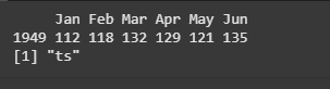
We can load the AirPassengers dataset and also check the class of the AirPassengers dataset to confirm it's a time series object, using the class function.

Output:

3. Box Plot for AirPassengers monthly count

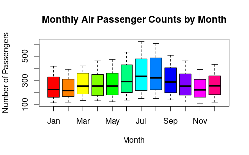
We can visualize the distribution of monthly passenger counts with a boxplot. Here, we use a custom color palette for better visualization.

Output:

4. Plotting the Time Series Data

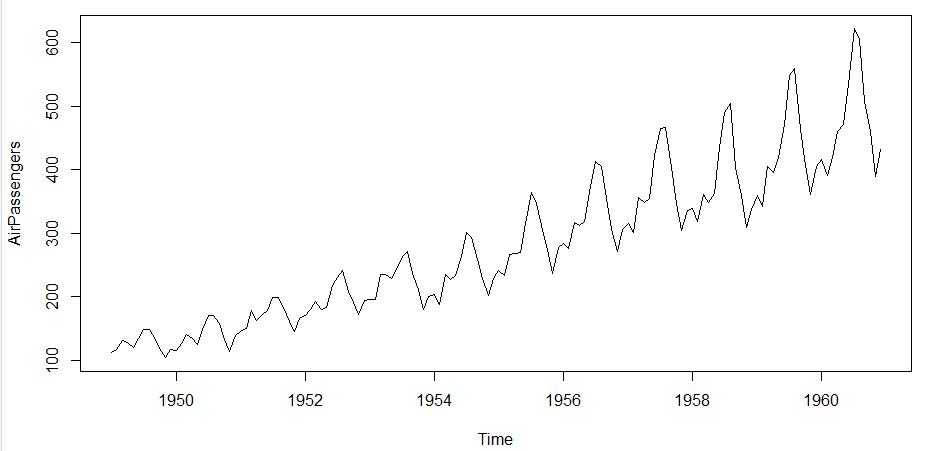
Next, we plot the AirPassengers data to observe trends and patterns over time.

Output:

The plot shows the passenger counts over time from 1949 to 1960, providing an initial look at the trend, seasonality and possible noise.

5. Decomposing the Time Series

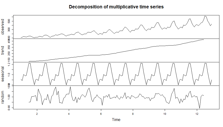
We will decompose the data using the "multiplicative" model, as the seasonal variation seems to change with the trend.

Output:

This plot shows the seasonal, trend and random components of the time series.

6. Forecasting with ARIMA

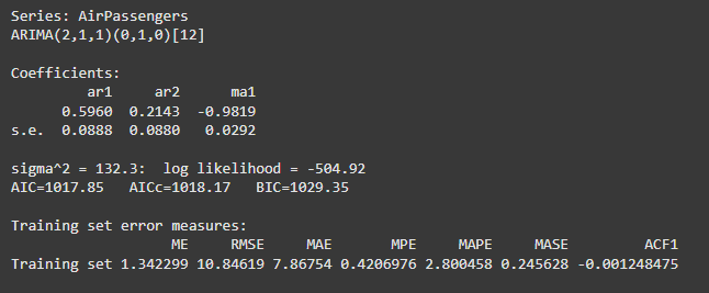
Now, we use the ARIMA model to forecast passenger data for the next 10 years (120 months). ARIMA is suitable for time series data that may have trends and seasonality.

Output:

The ARIMA(2,1,1)(0,1,0)[12] model includes:

• AR(2): Two autoregressive terms.
• I(1): First-order differencing to make the series stationary.
• MA(1): A first-order moving average term.
• Seasonal component (12): A seasonal period of 12 months.

7. Forecasting the Next 10 Years

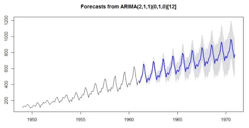
We forecast passenger counts for the next 10 years (120 months) using the ARIMA model.

Output:

The forecast provides the predicted number of passengers for each month from 1960 to 1970. The shaded area in the plot represents the 95% confidence interval for the forecast, indicating the level of uncertainty in the predictions.

Packages for Time Series Forcasting in R

In R Programming Language There are several R packages available for time series forecasting, including.

1. "forecast": This package provides a wide range of methods for time series forecasting, including exponential smoothing, ARIMA and neural networks.
2. "tseries": This package provides functions for time series analysis and forecasting, including functions for decomposing time series data and for fitting and forecasting models such as ARIMA.
3. "prophet": This package is developed by Facebook, it provides a simple and fast way to perform time series forecasting using additive models. It is designed for business time-series data and it is easy to interpret and to use.
4. "rugarch": This package provides a flexible framework for fitting and forecasting volatility models, including GARCH and its variants.
5. "stlplus": This package provides functions for decomposing time series data using the STL algorithm which is useful for removing seasonal and trend components from time series data.

To use these packages, first, they need to be installed and loaded into R. Then, the time series data must be prepared and cleaned and the appropriate forecasting method can be applied. The forecasted values can then be plotted, evaluated and compared to the actual values.